Week 5.1 - Mid term project - Solving the steady and unsteady 2D heat conduction problem
AIM -Solve the 2D heat conduction equation using point iterative techniques -Steady-state and transient state analysis (implicit and explicit).
GIVEN CONDITIONS
Top Boundary = 600 K
Bottom Boundary = 900 K
Left Boundary = 400 K
Right Boundary = 800 K
Absolute Error Criteria =1e-4
SOLUTION
Steady State Equation
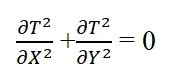
Firstly we describe the steady-state equation so that it can be solved using Matlab by Jacobi, Gauss-Siedel, and Successive method of discretizing the steady-state equation.
We define the grid point n = 50 and assume the no. of grid points in x and y directions are equal i.e ny=nx i.e the plate is square of length 1m. Then we define the temperature of 300K over the plate and applying the boundary temperature as per the given data. The absolute error criteria are assumed to be 1e-4. The error is checked after each iteration and the loop continues till the error obtained is less than the error assumed (used as 'tol' in the program).
Iterative Techniques
1) Jacobi Iterations
The formula used is as below
T(i,j)=term*((T_old(i-1,j)+T_old(i+1,j))/(dx^2)+(T_old(i,j-1)+T_old(i,j+1))/(dy^2));
where term is calculated using ''term=(dx^2*dy^2)/(2*(dx^2+dy^2))''
2) Guass Siedel Iteration
The formula used is as below
T(i,j)=term*((T(i-1,j)+T_old(i+1,j))/(dx^2)+(T(i,j-1)+T_old(i,j+1))/(dy^2));
where term is calculated using ''term=(dx^2*dy^2)/(2*(dx^2+dy^2))''
3) Successive over Relaxation method
The formula used is as below
T(i,j)=term*((T(i-1,j)+T_old(i+1,j))/(dx*dx)+(T(i,j-1)+T_old(i,j+1))/dy^2);
T(i,j)=T_old(i,j)*(1-omega)+(omega*(T(i,j)));
where term is calculated using ''term=(dx^2*dy^2)/(2*(dx^2+dy^2))'' and omega =1.8
CODE
Program
L=1; %Length
nx=50; % No. of grid point
ny=nx;

x=linspace(0,L,nx);
dx=x(2)-x(1);
y=linspace(0,L,ny);
dy=y(2)-y(1);

% Temperature Matrix
T=300*ones(ny,nx);
T(:,1)=400;
T(1,:)=600;
T(:,end)=800;
T(end,:)=900;

T_old=T;

term=(dx^2*dy^2)/(2*(dx^2+dy^2));
tol=1e-4; % Absolute Error
err=1;  % Initial Assumed Value of Error
iteration_method=1;
if iteration_method ==1 %Jacobi Iteration
tic
iter=0;
while(err>tol)
    for j= 2:ny-1
        for i=2:nx-1
            T(i,j)=term*((T_old(i-1,j)+T_old(i+1,j))/(dx^2)+(T_old(i,j-1)+T_old(i,j+1))/(dy^2));
        end
    end
    err=max(max(abs(T-T_old)));
    T_old=T;
    iter =iter+1;
end
time=toc;

elseif iteration_method ==2 %Guass Siedel
  omega=1.8;
  tic
  iter=0;
  while(err>tol)
    for j= 2:ny-1
        for i=2:nx-1
            T(i,j)=term*((T(i-1,j)+T_old(i+1,j))/(dx^2)+(T(i,j-1)+T_old(i,j+1))/(dy^2));
        end
    end
    err=max(max(abs(T-T_old)));
    T_old=T;
    iter =iter+1;
  end
  time=toc;

  elseif iteration_method == 3; %Successive Method
      omega=1.8;
  tic
  iter=0;
  while(err>tol)
    for j= 2:ny-1
        for i=2:nx-1
           T(i,j)=term*((T(i-1,j)+T_old(i+1,j))/(dx*dx)+(T(i,j-1)+T_old(i,j+1))/dy^2);
           T(i,j)=T_old(i,j)*(1-omega)+(omega*(T(i,j)));
        end
    end
    err=max(max(abs(T-T_old)));
    T_old=T;
    iter =iter+1;
  end
  time =toc;
end
  [c,h]=contourf(x,y,T);
  clabel(c,h)
  colorbar
  colormap(jet)
  ax = gca;
  ax.YDir='reverse';
  grid on
  xlabel('X Axis');
  ylabel ('Y Axis');
  title({'Steady state Temperature';['Iteration Method =',num2str(iteration_method)];['Number of Iterations =',num2str(iter)];['Simulation time =',num2str(time)]});
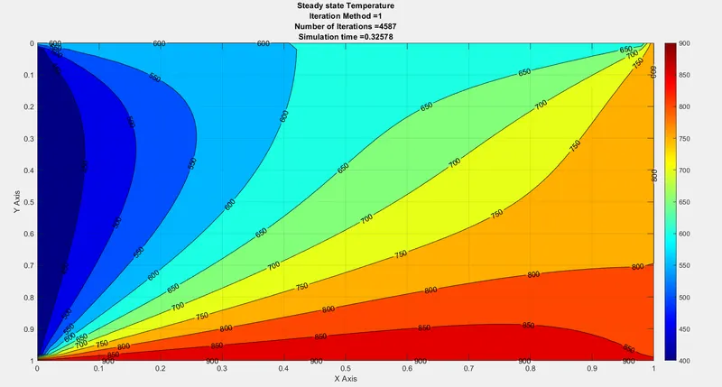
Fig (1) Jacobi Iteration
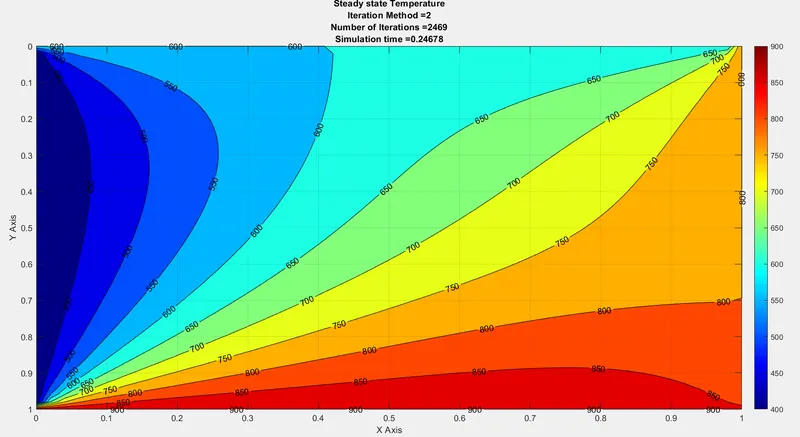
Fig 2 Guass Siedel Iteration
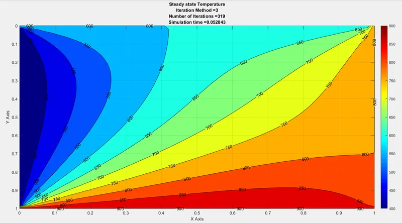
Fig 3 Successive over relaxation method
Conclusion
From the above three iterations plot it is clear that simulation time as well as no. of iterations is in the following sequence
Successive over relaxation < Guass Sieldel < Jacobi Iteration
TRANSIENT 2D HEAT CONDUCTION
The heat conduction is represented below (Transient Condition)
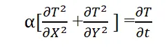
Equation for Explicit
n=100 (grid size)
Using Forward differencing method for time derivative and central differencing for space derivative

As we are solving explicitly n is on the RHS side.
CODE
L=1;
nx=100;
ny=nx;
dt=0.14;
t=200;
nt=t/dt;
alpha=1.75e-4;

x=linspace(0,L,nx);
dx=x(2)-x(1);
y=linspace(0,L,ny);
dy=y(2)-y(1);
CFL=alpha*dt*((1/dx^2)+(1/dy^2))

T=300*ones(ny,nx);
T(:,1)=400;
T(1,:)=600;
T(:,end)=800;
T(end,:)=900;
T_old=T;

k1=alpha*dt/dx^2;
k2=alpha*dt/dy^2;
 for k=1:nt
     for j=2:ny-1
         for i=2:nx-1
             H=(T_old(i-1,j)-2*T_old(i,j)+T_old(i+1,j));
             V=(T_old(i,j-1)-2*T_old(i,j)+T_old(i,j+1));
             T(i,j)=T_old(i,j)+(H*k1)+(V*k2);
         end
     end
     T_old=T;
     iter=iter+1;
 end
 time=toc
  [c,h]=contourf(x,y,T);
  clabel(c,h)
  colorbar
  colormap(jet)
  ax = gca;
  ax.YDir='reverse';
  grid on
  title({'Transient state Explicit temperature Profile';['Simulation time =',num2str(time)];['CFL=',num2str(CFL)]});
PLOT
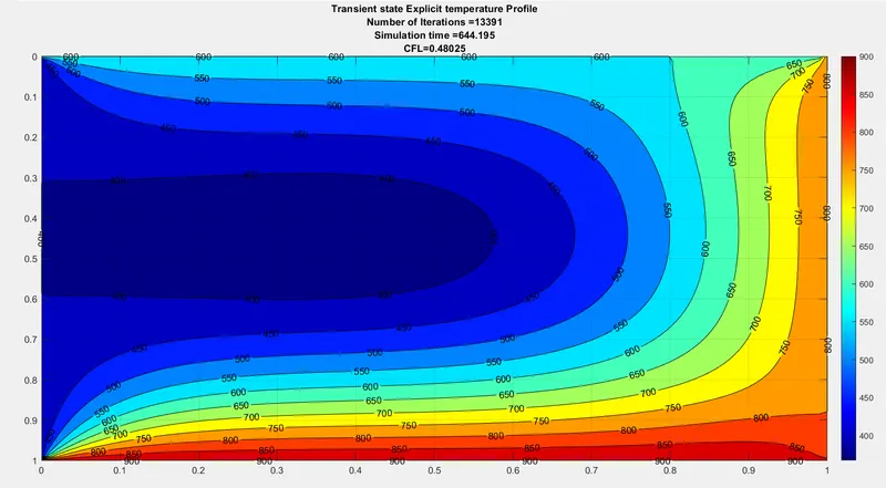
FIG 4 Transient state Explicit Temperature Profile (t = 200)
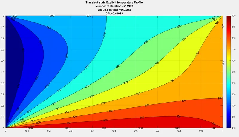
FIG 5 Transient state Explicit Temperature Profile (t = 1000)
Both the plot shows that the value of 't' increase no. of iterations as well as the simulation time increase.
IMPLICIT SOLUTION
Applying forward differencing to time derivative and central differencing to space derivative we get

The term (n+1) is on the RHS side
CODE
L=1;
nx=100;% Grid points
ny=nx;
t=200;
dt=10;
nt=t/dt;
alpha=1.75e-4;


x=linspace(0,L,nx);
dx=x(2)-x(1);
y=linspace(0,L,ny);
dy=y(2)-y(1);
CFL=alpha*dt*((1/dx^2)+(1/dy^2));
% Temperature Matrix
T=300*ones(ny,nx);
T(:,1)=400;
T(1,:)=600;
T(:,end)=800;
T(end,:)=900;

T_old=T;
T_prev=T;
k1=alpha*dt/dx^2;
k2=alpha*dt/dy^2;

tol=1e-4; % Error
err=1; % Intial assumed error

iteration_method=1;

if iteration_method ==1 %JACOBI METHOD
tic
iter=1;
for k=1:nt
    err=1;
    while err > tol
        for j= 2:ny-1
            for i=2:nx-1
                term1=1/(1+2*k1+2*k2);
                term2=k1*term1;
                term3=k2*term1;
                H=(T_old(i-1,j)+T_old(i+1,j));
                V=(T_old(i,j-1)+T_old(i,j+1));
                T(i,j)=(T_prev(i,j)*term1)+(H*term2)+(V*term3);
            end
        end
        err=max(max(abs(T-T_old)));
        T_old=T;
        iter =iter+1;
    end
    T_prev=T;
end
time=toc;

elseif iteration_method ==2 % Guass siedel
    tic
iter=1;
for k=1:nt
    err=1;
    while err > tol
        for j= 2:ny-1
            for i=2:nx-1
                term1=1/(1+2*k1+2*k2);
                term2=k1*term1;
                term3=k2*term1;
                H=(T(i-1,j)+T_old(i+1,j));
                V=(T(i,j-1)+T_old(i,j+1));
                T(i,j)=(T_prev(i,j)*term1)+(H*term2)+(V*term3);
            end
        end
        err=max(max(abs(T-T_old)));
        T_old=T;
        iter =iter+1;
    end
    T_prev=T;
end
time=toc;


  elseif iteration_method == 3; % Succerive over relaxation
      omega=1.1;
  tic
  iter=1;
  tic
iter=1;
for k=1:nt
    err=1;
    while err > tol
        for j= 2:ny-1
            for i=2:nx-1
                term1=1/(1+2*k1+2*k2);
                term2=k1*term1;
                term3=k2*term1;
                H=(T(i-1,j)+T_old(i+1,j));
                V=(T(i,j-1)+T_old(i,j+1));
                T(i,j)=(T_prev(i,j)*term1)+(H*term2)+(V*term3);
                T(i,j)=T_old(i,j)*(1-omega)+omega*T(i,j);
            end
        end
        err=max(max(abs(T-T_old)));
        T_old=T;
        iter =iter+1;
    end
    T_prev=T;
end
time=toc;
end
  [c,h]=contourf(x,y,T);
  clabel(c,h)
  colorbar
  colormap(jet)
  ax = gca;
  ax.YDir='reverse';
  grid on
  title({'Transient State Implicit Temperature Profile';['Iteration Method =',num2str(iteration_method)];['Number of Iterations =',num2str(iter), 'Time=',num2str(t)];['Simulation time =',num2str(time)];['CFL=',num2str(CFL)]});
PLOT
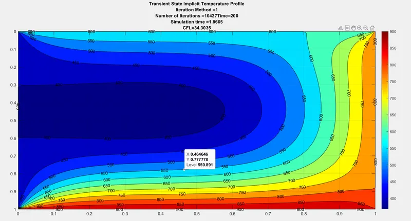
FIG 6 IMPLICIT TRANSIENT 2D HEAT CONDUCTION (JACOBI)
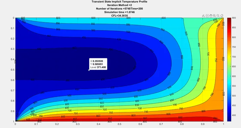
FIG 7 IMPLICIT TRANSIENT 2D HEAT CONDUCTION (GUASS SIEDEL)
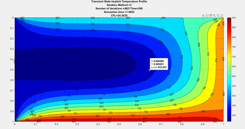
FIG 7 IMPLICIT TRANSIENT 2D HEAT CONDUCTION (Successive over-relaxation)
COMMENT
1. The plot observed in implicit and explicit transient 2D Heat conduction is the same (t=200)
2. From the above three iterations plot, it is clear that simulation time as well as no. of iterations is in the following sequence - Successive over-relaxation < Guass Sieldel < Jacobi Iteration