Week 3 - Taylor table method and Matlab code

DERIVE THE FOURTH ORDER APPROXIMATION OF SECOND ORDER DERIVATIVE

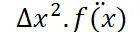
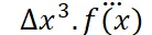
SKEWED RIGHT SIDED DIFFERENCE

	f(x)
a.f(i)	a	0	0	0	0	0
b.f(i+1)	b	b	b/2	b/6	b/24	b/120
c.f(1+2)	c	2c	4c/2	8c/6	16c/24	32c/120
d.f(i+3)	d	3d	9d/2	27d/6	27d/6	243d/120
e.f(i+4)	e	4e	16e/2	64e/6	64e/6	1024e/120
g.f(i+5)	g	5g	25g/2	125g/6	625g/24	3125g/120
SUM	0	0	1	0	0	0

SKEWED LEFT SIDED DIFFERENCE

	f(x)	.
a.f(i)	a	0	0	0	0	0
b.f(i-1)	b	-b	b/2	-b/6	b/24	-b/120
c.f(i-2)	c	-2c	4c/2	-8c/6	16c/24	-32c/120
d.f(i-3)	d	-3d	9d/2	-27d/6	27d/6	-243d/120
e.f(i-4)	e	-4e	16e/2	-64e/6	64e/6	-1024e/120
g.f(i-5)	g	-5g	25g/2	-125g/6	625g/24	-3125g/120
SUM	0	0	1	0	0	0

CENTRAL DIFFERENCE

	f(x)
a.f(i-1)	a	-2a	4a/2	-8a/6	16a/24
b.f(i-2)	b	-b	b/2	-b/6	b/24
c.f(i)	c	0	0	0	0
d.f(i+1)	d	d	d/2	d/6	d/24
e.f(i+2)	e	2e	4e/2	8e/6	16e/24
SUM	0	0	1	0	0

Solving the matrix represented in above tables to find values of a,b,c,d,e

For central Differencing

[A] =[1 1 1 1 1 1 ; -2 1 0 1 2; 2 0.5 0 0.5 2; -4/3 -1/6 0 1/6 4/3; 2/3 1/24 0 1/24 2/3]

[B] =[0;0;1;0;0]

X=A\B

Solving the above equation using Matlab to find a, b, c, d, e using linsolve function

MATLAB CODE

% Central Difference Skewed Approximation
[S]=[1 1 1 1 1 ; -2 -1 0 1 2; 2 1/2 0 1/2 2; -8/6 -1/6 0 1/6 8/6; -16/24 1/24 0 1/24 16/24];

[U]=[0;0;1;0;0];

X=linsolve(S,U);

% Right Hand Skewed Fourth Order Approximation
[H]=[1 1 1 1 1; 0 1 2 3 4 ; 0 1/2 2 9/2 8; 0 1/6 4/3 9/2 32/3; 0 1/24 2/3 27/8 32/3];
 
 [A]=[0;0;1;0;0];
 
 Y=linsolve(H,A);
 
 % Left-Handed Difference Fourth Order Approximation
 [N]=[1 1 1 1 1 ; 0 -1 -2 -3 -4 ; 0 1/2 2 9/2 8; 0 -1/6 -4/3 -9/2 -32/3; 0 1/24 2/3 27/8 32/3];
 
 [K]=[0;0;1;0;0];
 
 Z=linsolve(N,K);
 
check_X =X(1)+X(2)+X(3)+X(4)+X(5);
check_central_difference=rats(X);
check_Y =Y(1)+Y(2)+Y(3)+Y(4)+Y(5);
check_skewed_right=rats(Y);
check_Z =Z(1)+Z(2)+Z(3)+Z(4)+Z(5);
check_skewed_left=rats(Z);

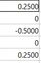
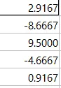
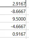
Values of a,b,c,d,e

For central Difference

For Right Hand Skewed Difference

For Left Hand Skewed Difference

MATLAB CODE

Main Program

x=pi/3;
dx=linspace(pi/10,pi/400,100);

Numerical=exp(x)*cos(x);
Derivative=-2*exp(x)*sin(x);

for i=1:length(dx)
    backward_difference(i)=(exp(x)*cos(x)-exp(x-dx(i))*cos(x-dx(i)))/dx(i);
    forward_difference(i)=(exp(x+dx(i))*cos(x+dx(i))-exp(x)*cos(x))/dx(i);
    
    b_error(i) = abs(backward_difference(i)-Derivative);
    f_error(i) = abs(forward_difference(i)-Derivative);
end

figure(1)
loglog(dx,b_error,'markerfacecolor','r','LineWidth',0.25)
hold on
loglog(dx,f_error,'markerfacecolor','b','LineWidth',0.25)
hold off
xlabel('dx')
ylabel('error')
legend('Backward Error','Forward Error','location','north')

x=pi/3;
dx=linspace(pi/4,pi/400,100)

func=exp(x)*cos(x);
derivative=-2*exp(x)*sin(x);

for i=1:length(dx)
    
    a(i)=(exp(x-(5*dx(i)))*cos(x-(5*dx(i))));
    b(i)=(exp(x-(4*dx(i)))*cos(x-(4*dx(i))));
    c(i)=(exp(x-(3*dx(i)))*cos(x-(3*dx(i))));
    d(i)=(exp(x-(2*dx(i)))*cos(x-(2*dx(i))));
    e(i)=(exp(x-(1*dx(i)))*cos(x-(1*dx(i))));
    f(i)=exp(x)*cos(x);
    g(i)=(exp(x+(1*dx(i)))*cos(x+(1*dx(i))));
    h(i)=(exp(x+(2*dx(i)))*cos(x+(2*dx(i))));
    j(i)=(exp(x+(3*dx(i)))*cos(x+(3*dx(i))));
    k(i)=(exp(x+(4*dx(i)))*cos(x+(4*dx(i))));
    l(i)=(exp(x+(5*dx(i)))*cos(x+(5*dx(i))));
    
    fourth_order_second_derivative_skewed_right(i) =(45*(f(i))-154*(g(i))+214*(h(i))-156*(j(i))+61*(k(i))-10*(l(i)))/(12*(dx(i)^2));
    fourth_order_second_derivative_skewed_left(i) =(45*(f(i))-154*(e(i))+214*(d(i))-156*(c(i))+61*(b(i))-10*(a(i)))/(12*(dx(i)^2));
    fourth_order_second_derivative_central_difference(i)=(-1*(d(i))+16*(e(i))-30*(f(i))+16*(g(i))-(h(i)))/(12*(dx(i)^2));
    
    fourth_order_skewed_right_error(i)=abs(fourth_order_second_derivative_skewed_right(i)-derivative)
    fourth_order_skewed_left_error(i)=abs(fourth_order_second_derivative_skewed_left(i)-derivative);
    fourth_order_central_difference_error(i)=abs(fourth_order_second_derivative_central_difference(i)-derivative);
end

figure(2)
loglog(dx,fourth_order_skewed_right_error,'-kd','markerfacecolor','b','markersize',10,'LineWidth',0.2)
hold on
loglog(dx,fourth_order_skewed_left_error,'-ks','markerfacecolor','y','markersize',10,'LineWidth',0.2)    
hold on
loglog(dx,fourth_order_central_difference_error,'-ko','markerfacecolor','r','markersize',10,'LineWidth',0.2)    
hold off
legend('fourth order skewed right error','fourth order skewed left error','fourth order central difference error','location','north')
xlabel('dx')
ylabel('error')
title('Comparision between different schemes of second order derivative of 4th order approximation ')

RESULT

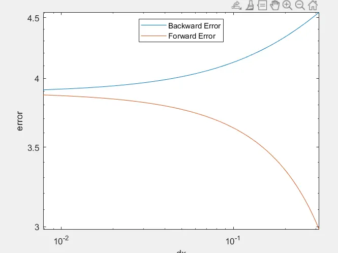
Figure(1)

Figure(2)

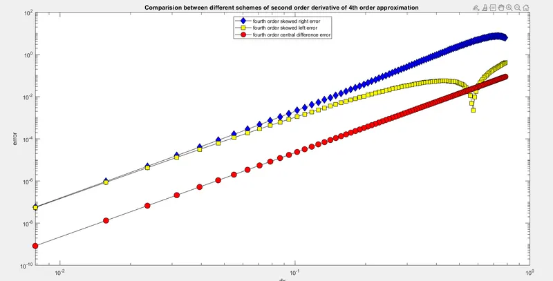
Figure (1) shows the plot of error in the forward scheme and backward scheme

Figure (2) shows the plot of error in right-skewed difference, left-skewed difference, and central difference v/s dx

Wy skewed scheme useful? What a skewed scheme can do which CD cannot?

In some complex systems, the numerical stencil won't be symmetric and at this point, only a skewed scheme can help. The advantage of using the skewed system can be seen near the boundaries where access to further points is unavailable over the boundary that is not symmetric.