Week 5.1 - Mid term project - Solving the steady and unsteady 2D heat conduction problem
Aim:-
To solve the steady & unsteady 2D heat conduction equation with the help of Jacobi , Gauss-siedel and sucessive over-relaxation by using the matlab code.
Theory:-
- Difference equations for the steady-state and unsteady-state 2D conduction equation are derived to obtain the numerical solution.
|
Steady State 2D heat conduction |
|
| Unsteady state Transient 2D heat conduction (explicit) | |
| Transient 2D heat conduction (implicit) |
- Here iterative methods are used to solve the difference equation, Iterative methods are numerical techniques used to converge the solution(accurately) of a problem with some initial guess.
- Here Jacobi, gauss-seidel, and successive over-relaxation techniques are used.
For simplicity, the subscripts are replaced as shown in the diagram :
The successive over relaxation method is an effective iterative solver. The SOR method uses either the solution obtained from jacobi method or from gauss seidel method. In additional to it, the relaxation factor(ω">ω�) is took in consider in case of SOR method.
Generally, In SOR --> Ti,j=(1-ω)Told+ω⋅">Ti,j=(1−ω)Told+ω⋅��,�=(1-�)����+�⋅(Final equation of either gauss seidel or jacobi method).
Matlab Code:-
> Here we will be using two codes in matlab for the execution for Steady state conduction and unsteady state conduction with same Input of data as shown below,
Inputs
| Top Boundary temperature | 600 K |
| Bottom Boundary temperature | 900 K |
| Left Boundary temperature | 400 K |
| Right Boundary temperature | 800 K |
| error | 1e-4 |
> While programming we will be assuming the Domain length shall be '' 1'' and No of grid points shall be ''10''
Steady-state 2D heat conduction:-
> All the inputs data are inserted with the variable.
> The BC with the temperature are shown in the form of array and the found the average of each temperature nodes at the four courner points
> Constant values are given for alpha,tolernace to run the iterative method
>we shall be using the command like for loop, while loop and if else for the iterative solution.
> Finally, the temperature distribution graph is obtained using 'conturf command'.
> Matlab code for Steady state:-
clear all
close all
clc

%inputs data
L=1 ; %Length
nx= 10 ; %No of grid points along in x-axis
ny=nx ;  %No of grid points along in y-axis
x=linspace(0,1,nx);
y=linspace(0,1,ny);
dx= x(2)-x(1);
dy=y(2)-y(1);

TL=400;  % Temperature at lower
TT=600;  % Temperature at top
TB=900;  % Temperature at bottom
TR=800;  % Temperature at right
T =300*ones(nx,ny);

%Temperature
T(1,2:ny-1)= TL ;
T(2:nx-1,ny)=TT ;
T(nx,2:ny-1)=TR ;
T(2:nx-1,1)=TB ;


% Calculating the AVG Temp @ corners
T(1,1)=(TT+TL)/2;
T(nx,ny)=(TB+TR)/2;
T(1,nx)=(TL+TB)/2;
T(1,ny)=(TT+TR)/2;


%Assigning the O.G value

T_old=T;

error=10;
tol=1e-4;

Iterative_solver=2;

 K = (2*(dx^2+dy^2))/(dx^2*dy^2);

 Omega=1.2;
% Jacobi method

if Iterative_solver==1
    jacobi_iter=1;

    while(error>tol)
        for i=2:nx-1
            for j=2:ny-1
             term1 = (T_old(i+1,j)+T_old(i-1,j))/dx^2;
            term2 = (T_old(i,j+1)+T_old(i,j-1))/dy^2;
            T(i,j) = (term1+term2)/K;
            end
    end
    error=max(max(abs(T_old-T)));
    T_old=T;
    jacobi_iter=jacobi_iter+1;
    end

% GS method

elseif Iterative_solver==2
    gs_iter=1;

    while(error>tol)
    for i=2:nx-1
        for j=2:ny-1
            term1 = (T_old(i+1,j)+T(i-1,j))/dx^2;
            term2 = (T_old(i,j+1)+T(i,j-1))/dy^2;
            T(i,j) = (term1+term2)/K;
         end
    end
    error=max(max(abs(T_old-T)));
   T_old=T;
    gs_iter=gs_iter+1;
    end
else
 Iterative_solver==3
    sos_iter=1;

    while(error>tol)
    for i=2:nx-1
        for j=2:ny-1
            term1 = (T_old(i+1,j)+T(i-1,j))/dx^2;
            term2 = (T_old(i,j+1)+T(i,j-1))/dy^2;
            T(i,j) = ((1-omegha)*T_old(i,j))+(omegha*((term1+term2)/K));
         end
end
   error=max(max(abs(T_old-T)));
   T=T_old;
    sos_iter=sos_iter+1;
    end
end
   plot(x,y);
   colormap(jet);
    contourf(x,y,T');
    colorbar;
    title('temperature distributor');
    xlabel('x-axis');
    ylabel('y-axis');
Plot for Gauss-seidel:-
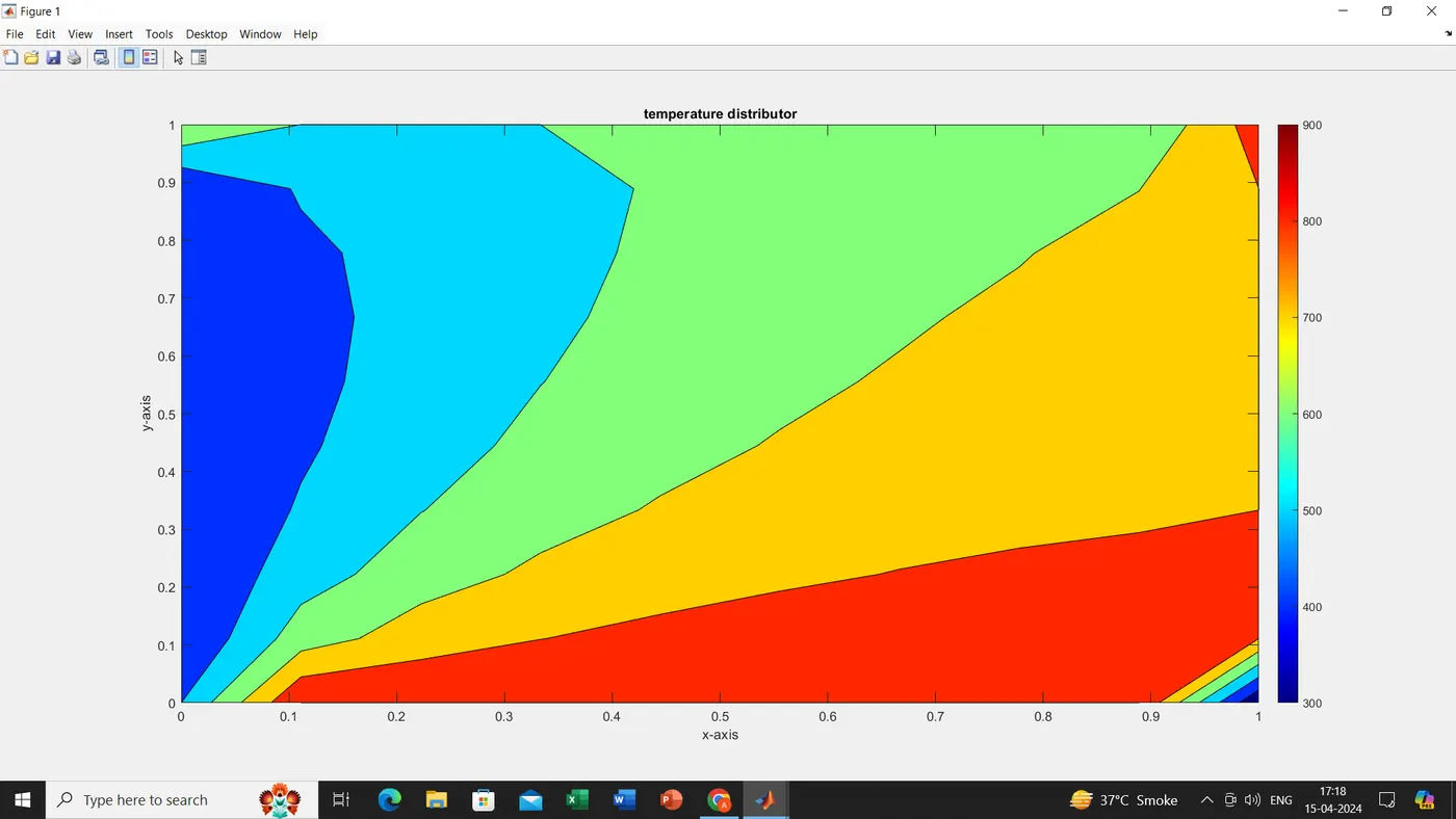
Similary we can solve for Jacobi and successive over-relaxation, only by changing the value for ''Iterative_solver''.
>Matlab code for unsteady code, explict
clear all
close all
clc

%inputs data
L=1 ; %Length
nx= 10 ; %No of grid points along in x-axis
ny=nx ;  %No of grid points along in y-axis
x=linspace(0,1,nx);
y=linspace(0,1,ny);
dx= x(2)-x(1);
dy=y(2)-y(1);
dt=0.01; %Time step
nt=500;  %No of time step


TL=400;  % Temperature at lower
TT=600;  % Temperature at top
TB=900;  % Temperature at bottom
TR=800;  % Temperature at right
T =300*ones(nx,ny);

%Temperature
T(1,2:ny-1)= TL ;
T(2:nx-1,ny)=TT ;
T(nx,2:ny-1)=TR ;
T(2:nx-1,1)=TB ;


% Calculating the AVG Temp @ corners
T(1,1)=(TT+TL)/2;
T(nx,ny)=(TB+TR)/2;
T(1,nx)=(TL+TB)/2;
T(1,ny)=(TT+TR)/2;


%
dt = 0.01; %time step
T_old=T;
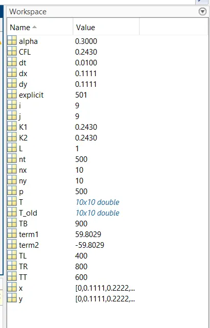
alpha = 0.3; % Thermal diffusivity

K1 = (alpha*dt)/(dx^2);
K2 = (alpha*dt)/(dy^2);
CFL = alpha*dt/(dx^2);

%EXPLICIT METHOD


    explicit = 1;
    for p = 1:nt
        for i = 2:nx-1
            for j = 2:ny-1
                term1 = (T_old(i-1,j)-2*T_old(i,j)+T_old(i+1,j));
                term2 = (T_old(i,j-1)-2*T_old(i,j)+T_old(i,j+1));
                T(i,j) = ((T_old(i,j))+(K1*term1)+(K2*term2));
            end
        end

    T_old=T;
    explicit = explicit+1;
    end


 %Plotting
    plot(x,y);
    colormap(jet);
    contourf(x,y,T,'showText','on');
    colorbar;
    title('temperature distributor');
    xlabel('x-axis');
    ylabel('y-axis');
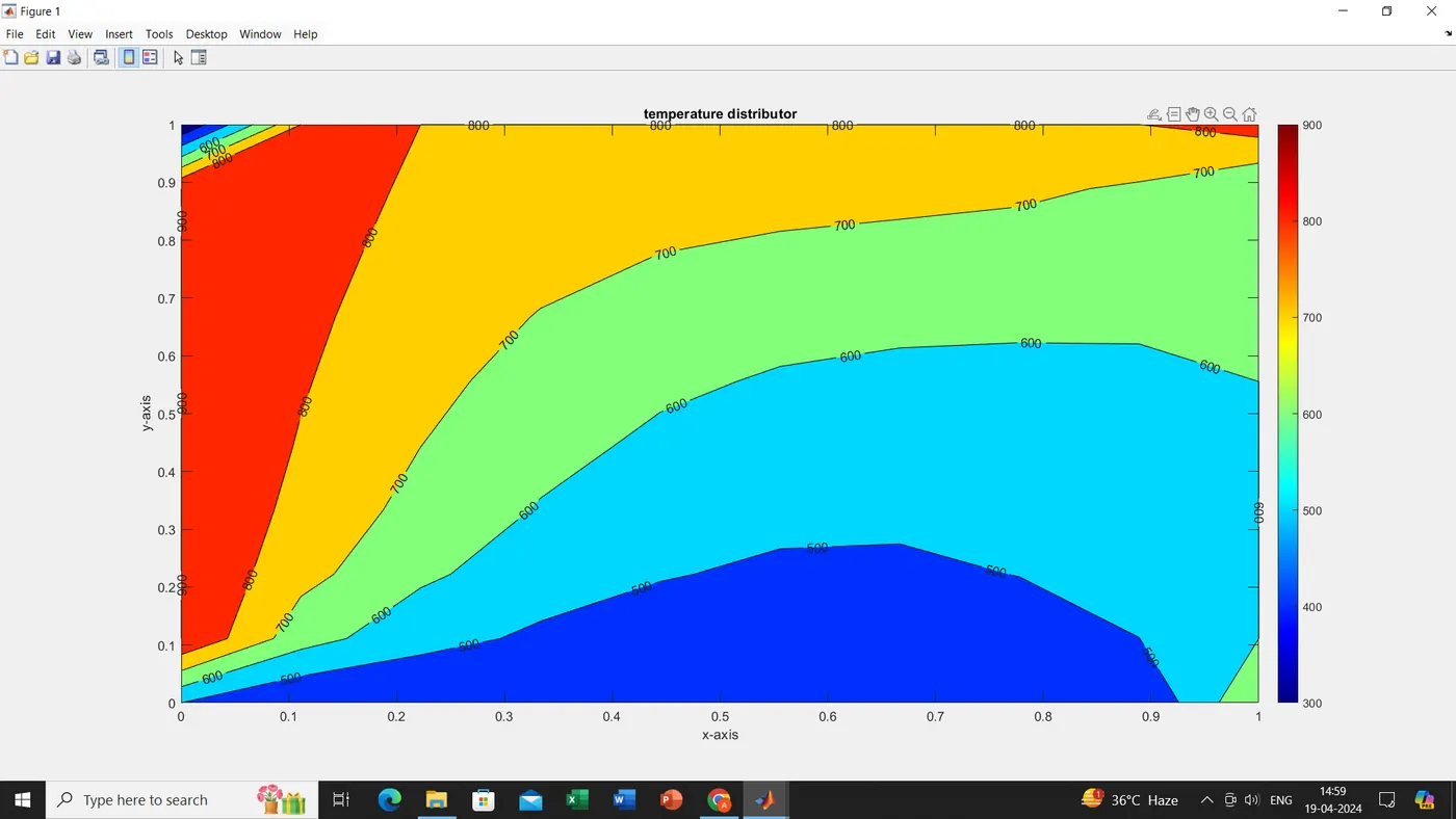
> Plot
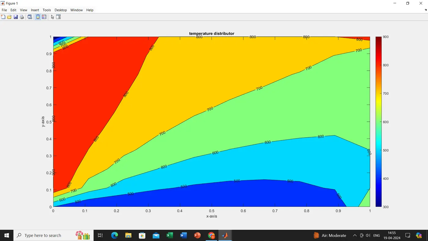
>Matlab code for Implict
clear all
close all
clc

%inputs data
L=1 ; %Length
nx= 10 ; %No of grid points along in x-axis
ny=nx ;  %No of grid points along in y-axis
x=linspace(0,1,nx);
y=linspace(0,1,ny);
dx= x(2)-x(1);
dy=y(2)-y(1);
dt=0.01; %Time step
nt=500;  %No of time step


TL=400;  % Temperature at lower
TT=600;  % Temperature at top
TB=900;  % Temperature at bottom
TR=800;  % Temperature at right
T =300*ones(nx,ny);

%Temperature
T(1,2:ny-1)= TL ;
T(2:nx-1,ny)=TT ;
T(nx,2:ny-1)=TR ;
T(2:nx-1,1)=TB ;


% Calculating the AVG Temp @ corners
T(1,1)=(TT+TL)/2;
T(nx,ny)=(TB+TR)/2;
T(1,nx)=(TL+TB)/2;
T(1,ny)=(TT+TR)/2;

%Assigning the O.G value

T_old=T;
Tprev_dt=T_old;
error=10;
tol=1e-4;

Iterative_solver=3;
omegha=1.2;
alpha=1;
k1=(alpha*dt)/(dx^.2);
k2=(alpha*dt)/(dy^.2);

% Jacobi method

if Iterative_solver==1

    jacobi_iter=1;
    for p=1:nt
        error=11
        while(error>tol)
        for i=2:nx-1
            for j=2:ny-1
                term1 = (1+(2*k1)+(2*k2))^-1;
                term2 = k1*term1;
                term3 = k2*term1;
                h = T_old(i-1,j)+T_old(i+1,j);
                v = T_old(i,j-1)+T_old(i,j+1);
                T(i,j) = (Tprev_dt(i,j)*term1)+(h*term2)+(v*term3);

            end
       end
       error=max(max(abs(T_old-T)));
    T_old=T;
    jacobi_iter=jacobi_iter+1;
        end
      Tprev_dt=T;
    end
% GS method
   elseif Iterative_solver==2
    gs_iter=1;

for p=1:nt
     error=11
        while(error>tol)
        for i=2:nx-1
            for j=2:ny-1
                term1 = (1+(2*k1)+(2*k2))^-1;
                term2 = k1*term1;
                term3 = k2*term1;
                h = T_old(i-1,j)+T_old(i+1,j);
                v = T_old(i,j-1)+T_old(i,j+1);
                T(i,j) = (Tprev_dt(i,j)*term1)+(h*term2)+(v*term3);

            end
end
    error=max(max(abs(T_old-T)));
    T_old=T;
     gs_iter=gs_iter+1;
        end
      Tprev_dt=T;
    end

% sos method
else Iterative_solver==3
    sos_iter=1;
for p=1:nt
     error=11
        while(error>tol)
        for i=2:nx-1
            for j=2:ny-1
                term1 = (1+(2*k1)+(2*k2))^-1;
                term2 = k1*term1;
                term3 = k2*term1;
                h = T_old(i-1,j)+T_old(i+1,j);
                v = T_old(i,j-1)+T_old(i,j+1);
                T(i,j)=((1-omegha)*T(i,j))+(omegha*((Tprev_dt(i,j)*term1)+(h*term2)+(v*term3)));
end
end
    error=max(max(abs(T_old-T)));
    T_old=T;
   sos_iter=sos_iter+1;
        end
      Tprev_dt=T;
    end
end
plot(x,y);
   colormap(jet);
    contourf(x,y,T,'showText','on');
    colorbar;
    title('temperature distributor');
    xlabel('x-axis');
    ylabel('y-axis');
> Plotting: