Week 5.1 - Mid term project - Solving the steady and unsteady 2D heat conduction problem
The problem statement and how we are applying implicit and explicit schemes for steady state and transient problems are written by hand and uploaded as a pdf.
First I wrote individual codes for different methods(Jacobi, G-S, SOR) of steady-state equation. After that, I tried to convert all of them into one MATLAB code so that it would be effective and time-saving. I did face some problems but was able to solve them.
Here is the code for a steady-state solver.
clear
close all
clc

% Parameters
nodes_x = 10;
nodes_y = 10;
T_l = 400;
T_r = 800;
T_t = 600;
T_b = 900;
error = 10;
tolerance = 1e-4;
alpha = 1.1;

% Jacobi Method
[T_jacobi, jacobi_iterations] = jacobi_solver(nodes_x, nodes_y, T_l, T_r, T_t, T_b, tolerance,error);

% Gauss-Seidel Method
[T_gs, gs_iterations] = gauss_seidel_solver(nodes_x, nodes_y, T_l, T_r, T_t, T_b, tolerance,error);

% Successive Over-Relaxation Method
[T_sor, sor_iterations] = sor_solver(nodes_x, nodes_y, T_l, T_r, T_t, T_b, tolerance, alpha,error);

% Plot Contours
figure;

% Plot filled contours of T for Jacobi Method
subplot(1, 3, 1);
contourf(linspace(0, 1, nodes_x), linspace(0, 1, nodes_y), T_jacobi);
colorbar;
colormap(jet);
set(gca, 'YDir', 'reverse');
xlabel('X-Axis');
ylabel('Y-Axis');
title('Contour plot using Jacobi method');

% Plot filled contours of T for Gauss-Seidel Method
subplot(1, 3, 2);
contourf(linspace(0, 1, nodes_x), linspace(0, 1, nodes_y), T_gs);
colorbar;
colormap(jet);
set(gca, 'YDir', 'reverse');
xlabel('X-Axis');
ylabel('Y-Axis');
title('Contour plot using Gauss-Seidel method');

% Plot filled contours of T for Successive Over-Relaxation Method
subplot(1, 3, 3);
contourf(linspace(0, 1, nodes_x), linspace(0, 1, nodes_y), T_sor);
colorbar;
colormap(jet);
set(gca, 'YDir', 'reverse');
xlabel('X-Axis');
ylabel('Y-Axis');
title('Contour plot using Successive Over-Relaxation method');


% Plot Iterations Comparison
% Define the methods and their corresponding iteration counts
methods = {'Jacobi', 'Gauss-Seidel', 'SOR'};
iterations = [jacobi_iterations, gs_iterations, sor_iterations];

% Print the iteration values in the command window
for i = 1:numel(methods)
    disp([methods{i}, ' method: ', num2str(iterations(i)), ' iterations']);
end

% Plot the bar graph
figure;
bar(categorical(methods), iterations);
ylabel('Number of Iterations');
title('Comparison of Iterations for Different Methods');

function [T, iterations] = jacobi_solver(nodes_x, nodes_y, T_l, T_r, T_t, T_b, tolerance,error)
    % Working area
    length = 1;

    % Discretization points
    x = linspace(0, length, nodes_x);
    y = linspace(0, length, nodes_y);

    % Mesh size
    dx = x(2) - x(1);
    dy = y(2) - y(1);

    % Initial guess at all nodes
    T = 100 * ones(nodes_x, nodes_y);

    % Temperature Boundary conditions
    T(2:nodes_y - 1, 1)  = T_l;
    T(2:nodes_y - 1, nodes_x) = T_r;
    T(1, 2:nodes_x - 1)  = T_t;
    T(nodes_y, 2:nodes_x - 1) = T_b;

    %To find the corner temperatures we will do the average to the right or
    %left or top or bottom based on the position
    T(1, 1) = (T_t + T_l) / 2;
    T(nodes_x, nodes_y) = (T_r + T_b) / 2;
    T(1, nodes_y) = (T_t + T_r) / 2;
    T(nodes_x, 1) = (T_l + T_b) / 2;

    %T values
    T_old = T;

    %k value
    k = (2 * (dx^2 + dy^2)) / ((dx^2) * (dy^2));

    % Jacobi iterative solver for steady state
    jacobi_ite = 1;

    while error>tolerance
        for i = 2:nodes_x - 1
            for j = 2:nodes_y - 1
                term1 = (T_old(i - 1, j) + T_old(i + 1, j)) / (dx^2);
                term2 = (T_old(i, j - 1) + T_old(i, j + 1)) / (dy^2);
                T(i, j) = (term1 + term2) / k;
            end
        end
        %error calculation
        error = max(max(abs(T_old - T)));
         jacobi_ite = jacobi_ite + 1;

        if error < tolerance
            break;
        end

        %reassigning the T and increasing iteration
        T_old = T;
    end

    iterations = jacobi_ite;
end

function [T, iterations] = gauss_seidel_solver(nodes_x, nodes_y, T_l, T_r, T_t, T_b, tolerance,error)
    % Working area
    length = 1;

    % Discretization points
    x = linspace(0, length, nodes_x);
    y = linspace(0, length, nodes_y);

    % Mesh size
    dx = x(2) - x(1);
    dy = y(2) - y(1);

    % Initial guess at all nodes
    T = 100 * ones(nodes_x, nodes_y);

    % Temperature Boundary conditions
    T(2:nodes_y - 1, 1)  = T_l;
    T(2:nodes_y - 1, nodes_x) = T_r;
    T(1, 2:nodes_x - 1)  = T_t;
    T(nodes_y, 2:nodes_x - 1) = T_b;

    %To find the corner temperatures we will do the average to the right or
    %left or top or bottom based on the position
    T(1, 1) = (T_t + T_l) / 2;
    T(nodes_x, nodes_y) = (T_r + T_b) / 2;
    T(1, nodes_y) = (T_t + T_r) / 2;
    T(nodes_x, 1) = (T_l + T_b) / 2;

    %T values
    T_old = T;

    %k value
    k = (2 * (dx^2 + dy^2)) / ((dx^2) * (dy^2));

    % Gauss-Seidel iterative solver for steady state
    gs_ite = 1;

    while error>tolerance
        for i = 2:nodes_x - 1
            for j = 2:nodes_y - 1
                term1 = (T(i - 1, j) + T_old(i + 1, j)) / (dx^2);
                term2 = (T(i, j - 1) + T_old(i, j + 1)) / (dy^2);
                T(i, j) = (term1 + term2) / k;
            end
        end
        %error calculation
        error = max(max(abs(T_old - T)));
         gs_ite = gs_ite + 1;

        if error < tolerance
            break;
        end

        %reassigning the T and increasing iteration
        T_old = T;

    end

    iterations = gs_ite;
end

function [T, iterations] = sor_solver(nodes_x, nodes_y, T_l, T_r, T_t, T_b, tolerance, alpha,error)
    % Working area
    length = 1;

    % Discretization points
    x = linspace(0, length, nodes_x);
    y = linspace(0, length, nodes_y);

    % Mesh size
    dx = x(2) - x(1);
    dy = y(2) - y(1);

    % Initial guess at all nodes
    T = 100 * ones(nodes_x, nodes_y);

    % Temperature Boundary conditions
    T(2:nodes_y - 1, 1)  = T_l;
    T(2:nodes_y - 1, nodes_x) = T_r;
    T(1, 2:nodes_x - 1)  = T_t;
    T(nodes_y, 2:nodes_x - 1) = T_b;

    %To find the corner temperatures we will do the average to the right or
    %left or top or bottom based on the position
    T(1, 1) = (T_t + T_l) / 2;
    T(nodes_x, nodes_y) = (T_r + T_b) / 2;
    T(1, nodes_y) = (T_t + T_r) / 2;
    T(nodes_x, 1) = (T_l + T_b) / 2;

    %T values
    T_old = T;

    %k value
    k = (2 * (dx^2 + dy^2)) / ((dx^2) * (dy^2));

    % Successive Over-Relaxation iterative solver for steady state
    sor_ite = 1;

    while error>tolerance
        for i = 2:nodes_x - 1
            for j = 2:nodes_y - 1
                term1 = (T(i - 1, j) + T_old(i + 1, j)) / (dx^2);
                term2 = (T(i, j - 1) + T_old(i, j + 1)) / (dy^2);
                T(i, j) = ((1 - alpha) * T_old(i, j)) + (alpha * (term1 + term2)) / k;
            end
        end
        %error calculation
        error = max(max(abs(T_old - T)));
        sor_ite = sor_ite + 1;

        if error < tolerance
            break;
        end

        %reassigning the T and increasing iteration
        T_old = T;

    end

    iterations = sor_ite;
end
Process:
1. Write the common parameters which are given as inputs for the function
2. Call each method with inputs
3. Plot the contours for all three methods and how many iterations each method took for the solution
4. Bar graph for the iterations
5. Functions where the methods are solved using the equations derived in the paper and from the lecture notes.
Here is the temperature result
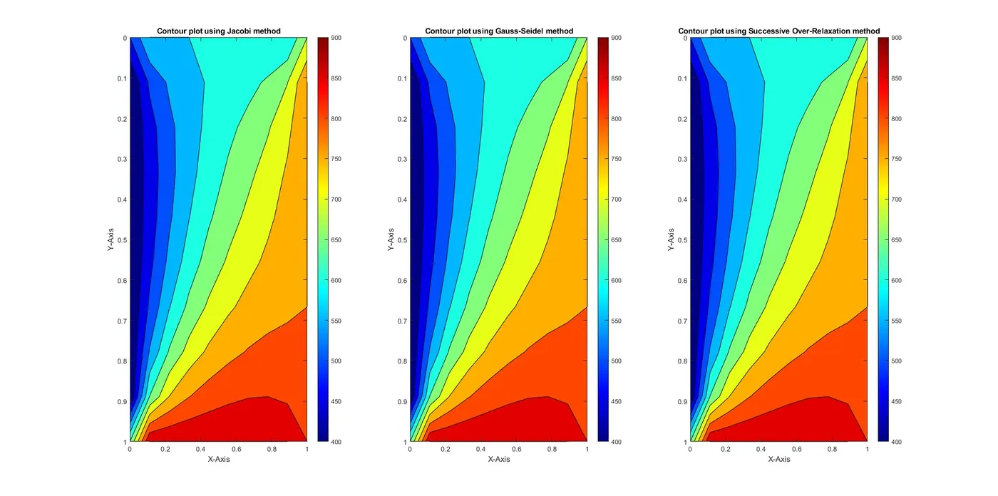
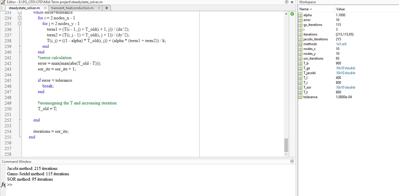
From these results, we can see that the temperature graphs are similar for each method but we can see the difference in how many iterations it took for each method. These iterations are shown in numbers and as a bar graph.
Here is the bar graph for the iterations.
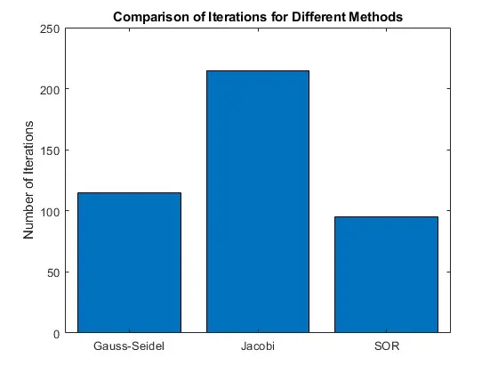
From these iterations, we can see that the SOR method took very less iterations for solving the same problem.
Now we will compare transient heat conduction problems using implicit and explicit schemes.
Implicit scheme: Same procedure as the steady state but the equations are different in terms of heat conduction.
For a time loop of 1000 iterations keeping the error at 10 and tolerance as mentioned in the problem. Here is the code for the transient heat conduction problem with time marching solution.
clear
close all
clc

% Parameters
nodes_x = 10;
nodes_y = 10;
T_l = 400;
T_r = 800;
T_t = 600;
T_b = 900;
error =10;
tolerance = 1e-4;
alpha = 1.1;
TD = 1.5;
dt =0.001;

% Jacobi Method
[T_jacobi, jacobi_iterations] = jacobi_solver(nodes_x, nodes_y, T_l, T_r, T_t, T_b, tolerance,error,dt,TD);

% Gauss-Seidel Method
[T_gs, gs_iterations] = gauss_seidel_solver(nodes_x, nodes_y, T_l, T_r, T_t, T_b, tolerance,error,dt,TD);

% Successive Over-Relaxation Method
[T_sor, sor_iterations] = sor_solver(nodes_x, nodes_y, T_l, T_r, T_t, T_b, tolerance, alpha,error,dt,TD);


% Plot Contours
figure;

% Plot filled contours of T for Jacobi Method
subplot(1, 3, 1);
contourf(linspace(0, 1, nodes_x), linspace(0, 1, nodes_y), T_jacobi);
colorbar;
colormap(jet);
set(gca, 'YDir', 'reverse');
xlabel('X-Axis');
ylabel('Y-Axis');
title('Contour plot using Jacobi method');

% Plot filled contours of T for Gauss-Seidel Method
subplot(1, 3, 2);
contourf(linspace(0, 1, nodes_x), linspace(0, 1, nodes_y), T_gs);
colorbar;
colormap(jet);
set(gca, 'YDir', 'reverse');
xlabel('X-Axis');
ylabel('Y-Axis');
title('Contour plot using Gauss-Seidel method');

% Plot filled contours of T for Successive Over-Relaxation Method
subplot(1, 3, 3);
contourf(linspace(0, 1, nodes_x), linspace(0, 1, nodes_y), T_sor);
colorbar;
colormap(jet);
set(gca, 'YDir', 'reverse');
xlabel('X-Axis');
ylabel('Y-Axis');
title('Contour plot using Successive Over-Relaxation method');


% Plot Iterations Comparison
% Define the methods and their corresponding iteration counts
methods = {'Jacobi', 'Gauss-Seidel', 'SOR'};
iterations = [jacobi_iterations, gs_iterations, sor_iterations];

% Print the iteration values in the command window
for i = 1:numel(methods)
    disp([methods{i}, ' method: ', num2str(iterations(i)), ' iterations']);
end

% Plot the bar graph
figure;
bar(categorical(methods), iterations);
ylabel('Number of Iterations');
title('Comparison of Iterations for Different Methods');

function [T, iterations] = jacobi_solver(nodes_x, nodes_y, T_l, T_r, T_t, T_b, ~,~,dt,TD)
    % Working area
    length = 1;

    % Discretization points
    x = linspace(0, length, nodes_x);
    y = linspace(0, length, nodes_y);

    % Mesh size
    dx = x(2) - x(1);
    dy = y(2) - y(1);

    % Initial guess at all nodes
    T = 100 * ones(nodes_x, nodes_y);

    % Temperature Boundary conditions
    T(2:nodes_y - 1, 1)  = T_l;
    T(2:nodes_y - 1, nodes_x) = T_r;
    T(1, 2:nodes_x - 1)  = T_t;
    T(nodes_y, 2:nodes_x - 1) = T_b;

    %To find the corner temperatures we will do the average to the right or
    %left or top or bottom based on the position
    T(1, 1) = (T_t + T_l) / 2;
    T(nodes_x, nodes_y) = (T_r + T_b) / 2;
    T(1, nodes_y) = (T_t + T_r) / 2;
    T(nodes_x, 1) = (T_l + T_b) / 2;

    %T values
    T_old = T;

     %k1 and k2 values
    k1=(TD*dt)/(dx^2);
   k2=(TD*dt)/(dy^2);

    % Jacobi iterative solver for Transient state
    jacobi_ite = 1;

  for nt = 1:1000
  error =10;
  tolerance = 1e-4;
    while error>tolerance
        for i = 2:nodes_x - 1
            for j = 2:nodes_y - 1
                term1 = 1/(1+(2*k1)+(2*k2));
                term2 = k1*(T_old(i - 1, j) + T_old(i + 1, j)) ;
                term3 = k2*(T_old(i, j - 1) + T_old(i, j + 1)) ;
                T(i, j) = (term1*((T_old(i, j)) + term2+term3));
            end
        end
        %error calculation
        error = max(max(abs(T_old - T)));
         jacobi_ite = jacobi_ite + 1;

        if error < tolerance
            break;
        end
        %reassigning the T and increasing iteration
        T_old = T;
    end
    iterations = jacobi_ite;

  end
end

function [T, iterations] = gauss_seidel_solver(nodes_x, nodes_y, T_l, T_r, T_t, T_b, ~,~,dt,TD)
    % Working area
    length = 1;

    % Discretization points
    x = linspace(0, length, nodes_x);
    y = linspace(0, length, nodes_y);

    % Mesh size
    dx = x(2) - x(1);
    dy = y(2) - y(1);

    % Initial guess at all nodes
    T = 100 * ones(nodes_x, nodes_y);

    % Temperature Boundary conditions
    T(2:nodes_y - 1, 1)  = T_l;
    T(2:nodes_y - 1, nodes_x) = T_r;
    T(1, 2:nodes_x - 1)  = T_t;
    T(nodes_y, 2:nodes_x - 1) = T_b;

    %To find the corner temperatures we will do the average to the right or
    %left or top or bottom based on the position
    T(1, 1) = (T_t + T_l) / 2;
    T(nodes_x, nodes_y) = (T_r + T_b) / 2;
    T(1, nodes_y) = (T_t + T_r) / 2;
    T(nodes_x, 1) = (T_l + T_b) / 2;

    %T values
    T_old = T;

     %k1 and k2 values
 k1=(TD*dt)/(dx^2);
 k2=(TD*dt)/(dy^2);

    % Gauss-Seidel iterative solver for Transient state
    gs_ite = 1;
for nt =1:1000
error =10;
tolerance =1e-4;
    while error>tolerance
        for i = 2:nodes_x - 1
            for j = 2:nodes_y - 1
                term1 = 1/(1+(2*k1)+(2*k2));
              term2 = k1*(T(i - 1, j) + T_old(i + 1, j)) ;
           term3 = k2*(T(i, j - 1) + T_old(i, j + 1)) ;
        T(i, j) = (term1*((T_old(i, j)) + term2+term3));
            end
        end
        %error calculation
        error = max(max(abs(T_old - T)));
         gs_ite = gs_ite + 1;

        if error < tolerance
            break;
        end

        %reassigning the T and increasing iteration
        T_old = T;

    end

    iterations = gs_ite;
end
end

function [T, iterations] = sor_solver(nodes_x, nodes_y, T_l, T_r, T_t, T_b, ~, alpha,~,dt,TD)
    % Working area
    length = 1;

    % Discretization points
    x = linspace(0, length, nodes_x);
    y = linspace(0, length, nodes_y);

    % Mesh size
    dx = x(2) - x(1);
    dy = y(2) - y(1);

    % Initial guess at all nodes
    T = 100 * ones(nodes_x, nodes_y);

    % Temperature Boundary conditions
    T(2:nodes_y - 1, 1)  = T_l;
    T(2:nodes_y - 1, nodes_x) = T_r;
    T(1, 2:nodes_x - 1)  = T_t;
    T(nodes_y, 2:nodes_x - 1) = T_b;

    %To find the corner temperatures we will do the average to the right or
    %left or top or bottom based on the position
    T(1, 1) = (T_t + T_l) / 2;
    T(nodes_x, nodes_y) = (T_r + T_b) / 2;
    T(1, nodes_y) = (T_t + T_r) / 2;
    T(nodes_x, 1) = (T_l + T_b) / 2;

    %T values
    T_old = T;

     %k1 and k2 values
 k1=(TD*dt)/(dx^2);
 k2=(TD*dt)/(dy^2);

    % SOR iterative solver for Transient state
    sor_ite = 1;
for nt =1:1000
error =10;
tolerance =1e-4;
    while error>tolerance
        for i = 2:nodes_x - 1
            for j = 2:nodes_y - 1
                term1 = 1/(1+(2*k1)+(2*k2));
              term2 = k1*(T(i - 1, j) + T_old(i + 1, j)) ;
           term3 = k2*(T(i, j - 1) + T_old(i, j + 1)) ;
        T(i, j) = (1-alpha)*T_old(i,j)+alpha*(term1*((T_old(i, j)) + term2+term3));
            end
        end
        %error calculation
        error = max(max(abs(T_old - T)));
         sor_ite = sor_ite + 1;

        if error < tolerance
            break;
        end

        %reassigning the T and increasing iteration
        T_old = T;

    end

    iterations = sor_ite;
end
end
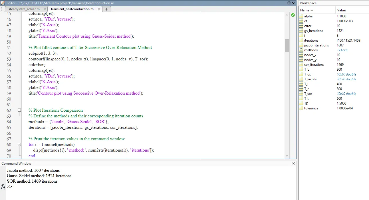
From this code, we can also see the temperature graph which will reveal that the temperature id going steady state and the graphs are all same.
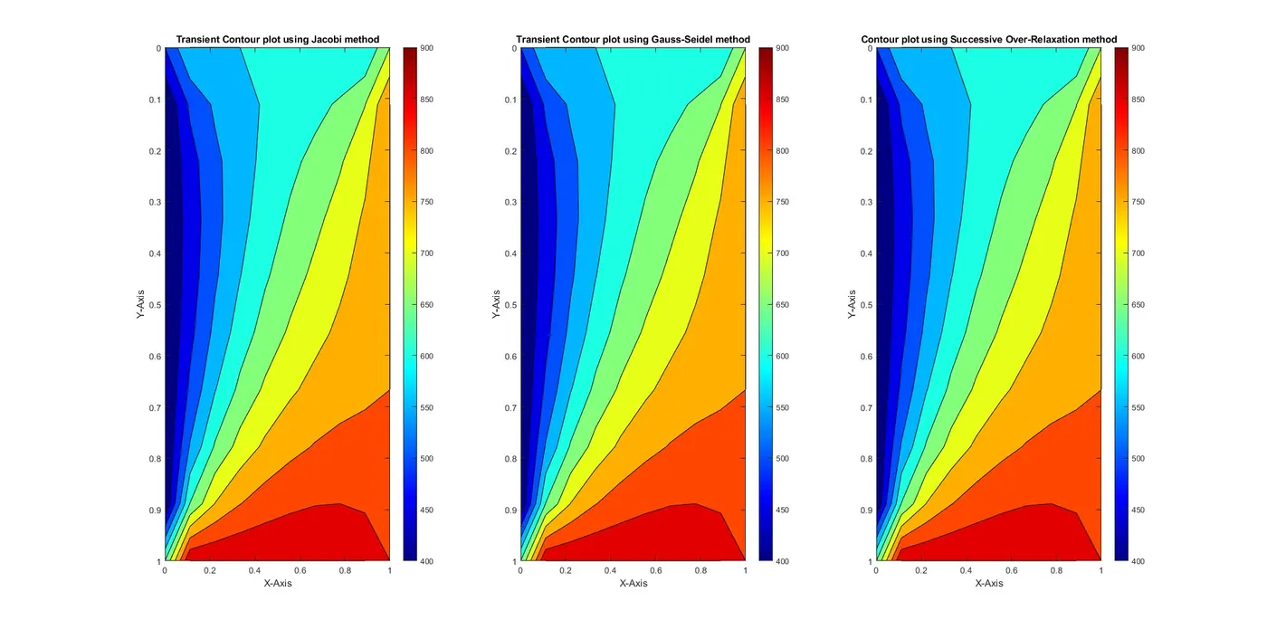
Now, we can look at the iterations in numbers and as a bar graph.
Bar Graph for iterations:
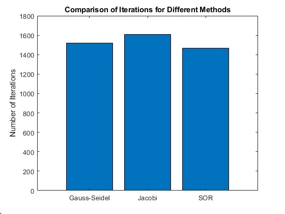
From this graph also we can observe that the SOR has a lesser no.of iterations compared with the other two methods at the same time.
Now let's take a look at an explicit solution
clear
close all
clc

% Parameters
nodes_x = 10;
nodes_y = 10;
length = 1;

% Discretization points
x = linspace(0, length, nodes_x);
y = linspace(0, length, nodes_y);

% Mesh size
dx = x(2) - x(1);
dy = y(2) - y(1);

% Error and tolerance
error = 10;
tolerance = 1e-4;
alpha = 1.5;
dt = 0.001;

% Temperature Boundary conditions
T_l = 400;
T_r = 800;
T_t = 600;
T_b = 900;

% Initial guess at all nodes
T = 100 * ones(nodes_x, nodes_y);

% Assigning the boundary conditions
T(2:nodes_y - 1, 1) = T_l;
T(2:nodes_y - 1, nodes_x) = T_r;
T(1, 2:nodes_x - 1) = T_t;
T(nodes_y, 2:nodes_x - 1) = T_b;

% To find the corner temperatures we will do the average to the right or
% left or top or bottom based on the position
T(1, 1) = (T_t + T_l) / 2;
T(nodes_x, nodes_y) = (T_r + T_b) / 2;
T(1, nodes_y) = (T_t + T_r) / 2;
T(nodes_x, 1) = (T_l + T_b) / 2;

% T values
T_old = T;

% Explicit iterative solver for Transient state
exp_ite = 1;

while error > tolerance
    T_new = T_old; % Copy the old temperature field

    for i = 2:nodes_x - 1
        for j = 2:nodes_y - 1
            term1 = T_old(i, j);
            term2 = alpha * (dt / dx^2) * (T_old(i + 1, j) - 2 * T_old(i, j) + T_old(i - 1, j));
            term3 = alpha * (dt / dy^2) * (T_old(i, j + 1) - 2 * T_old(i, j) + T_old(i, j - 1));
            T_new(i, j) = term1 + term2 + term3;
        end
    end

    % Error calculation
    error = max(max(abs(T_old - T_new)));

    % Update T_old
    T_old = T_new;

    % Increment iteration count
    exp_ite = exp_ite + 1;

end
% Display total number of iterations
disp(['Total number of iterations in Explicit scheme: ', num2str(exp_ite)]);


% Plot contours of T for Explicit Method
figure;
contourf(linspace(0, 1, nodes_x), linspace(0, 1, nodes_y), T_old);
colorbar;
colormap(jet);
set(gca, 'ydir', 'reverse');
xlabel('X-Axis');
ylabel('Y-Axis');
title('Contour plot using Explicit method');
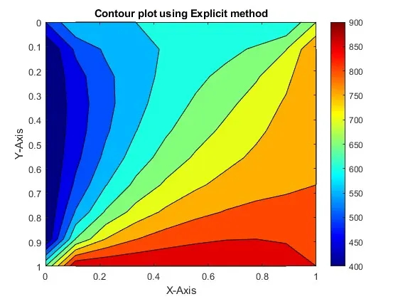
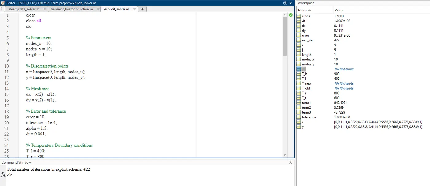
From the explicit scheme approach, we can see that the no.of iterations is far better than the implicit schemes. here is the graph for the temperature and the screenshot for the no.of iterations.
Outcomes:
1. The SOR method is the most effective method from the point of view of the number of iterations.
2. Comparing Transient and steady state, the steady state took less number of iterations.