Week 5.1 - Mid term project - Solving the steady and unsteady 2D heat conduction problem
Numerical Solution of 2D Heat Conduction Equation
Objective
The primary objective of this project is to solve both the steady and the transient 2D Heat Conduction using Finite Difference Method on a rectangular domain. The transient equation was solved using implicit and explicit methods. Iterative solvers were used where possible. In the end, the results were visualized.
Theory
The general transient heat conduction equation is represented by the following equation:
`(dT)/(dt) – alpha*nabla^2T = 0 ` ----------------------------------------- (1)
Where `T` represents the temperature, `t` the time, `alpha` the diffusion coefficient and `nabla^2` is the diffusion operator. The general value of `alpha` will be of the order of `10^(-5)`[1] which is very low and it will take longer time to simulate the same numerically. Hence, an artificial diffusion coefficient of 0.5 was selected here.
In 2D the equation (1) will be transformed to the following equation:
`(dT)/(dt) – alpha*((d^2T)/(dx^2) + (d^2T)/(dy^2)) = 0` -------------------(2)
The finite difference method was applied here to solve the equation numerically. The above equation (1) is a parabolic equation [2] and therefore, the time derivative was discretized using the Forward Euler Method and the space derivatives (in x and y) were discretized using a 2nd order accurate Central Differencing Method. The CDM was used because of the inherent characteristic of the parabolic equation– infinite speed of propagation of information [2].
The schematic representation of the stencil used for discretizing the space derivatives is shown in the figure below where P represents the point of interest and L,R,T,B represents the neighbouring points
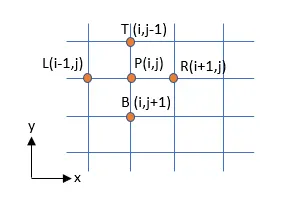
The linear system of equations were solved using 3 different iterative solvers (expect the explicit method as it does not produce a system of equations).
- Jacobi Method
The Jacobi method is a method of solving a matrix equation (`A*x = b` ) that has no zeros along its main diagonal. Each diagonal element is solved for, starting with an approximate initial values. The process is then iterated until the solution converges [3].
In isolation, the ith equation can be written as
`sum_(j=1)^N a_(i,j)*x_j = b_i`
The value for `x_i` can be solved iteratively with the assumption that other `x` remain fixed.
`x_i^(k) = (b_j – sum_(i != j) a_(i,j)*x_j^(k-1) )/a_(i,i)`
Where k represents the current iteration. The iteration continue until the abs(x^k – x^(k-1)) is less than a specified tolerance.
- Gauss-Seidel (GS) Method
The Gauss-Seidel Method is also an iterative method for solving the system of n linear equations (`A*x = b` ). The main difference between this method and the jacobi method is that the GS method uses the previously computed values as soon as possible. That is, when `x_i` is being calculated, the value of `x_(i-1)` is already known and it is used in the calculation of `x_i` in the same iteration [4].
`x_i^(k) = (b_j – sum_(j < i) a_(i,j)*x_j^(k) - sum_(j > i) a_(i,j)*x_j^(k-1) )/a_(i,i)`
- Successive Over Relaxation (SOR) Method
The SOR method is an extrapolation of the Gauss-Seidel Method which is a result of taking the weighted average between the previous iterate value and the calculated GS value [5].
`x_i^k = omega*(bar x)_i^k + (1-omega)* x_i^(k-1)`
Where `bar x` denotes the GS value and `omega` is the extrapolation factor. The idea is to chose `omega` such that the convergence to solution is accelerated. When `omega=1`, the method reduces to the GS method. A study by kahan shows that the SOR method fails when `omega` exceeds the range of (0,2).
Implementation,Results and Discussion:
Steady-State Solution
Under steady-state, the time derivative vanishes and only the space derivative will be remaining.
`(d^2T)/(dx^2) + (d^2T)/(dy^2) = 0` ------------------------------- (3)
The above equation is discretized using the CDM scheme and results in the following difference equation:
`(T(i+1,j) – 2* T(I,j) + T(i-1,j))/( Deltax ^2) + (T(i+1,j) – 2* T(I,j) + T(i-1,j))/( Deltay ^2) = 0`
`(T_L – 2*T_P + T_R)/( Deltax ^2) + (T_T – 2*T_P + T_B)/( Deltay ^2) = 0`
`T_P * (2*(Deltax^2 + Deltay^2)/(Deltax^2*Deltay^2)) = (T_L +T_R)/(Deltax^2) + (T_T + T_B)/(Deltay^2)`
The above linear system of equations were solved iteratively using the previously defined iterative methods. These methods were implemented using the following functions
function [T_solved,err,iter_jacobi] = jacobi(T,x,y,tol)

    dx = x(2) - x(1);
    dy = y(2) - y(1);
    nx = length(x);
    ny = length(y);
    k = 2.*(dx.^2 + dy.^2)./(dx^2.*dy^2);

    err = 9e9;

    iter_jacobi = 1;
    while(err > tol)
        Told = T;
        for i = 2:nx-1
            for j = 2:ny-1
                T(i,j) = (1./k).*(Told(i-1,j) + Told(i+1,j))/dx.^2 + (1./k).*(Told(i,j-1) + Told(i,j+1))/dy.^2;
            end
        end

        err = sum(max(abs(T - Told)));
        iter_jacobi = iter_jacobi + 1;

    end
    T_solved = T;

end

% Gauss-Seidel Method
function [T_solved,err,iter_gs] = GS(T,x,y,tol)

    dx = x(2) - x(1);
    dy = y(2) - y(1);
    nx = length(x);
    ny = length(y);
    k = 2.*(dx.^2 + dy.^2)./(dx^2.*dy^2);

    err = 9e9;

    iter_gs = 1;
    while(err > tol)
        Told = T;
        for i = 2:nx-1
            for j = 2:ny-1
                T(i,j) = (1./k).*(T(i-1,j) + Told(i+1,j))/dx.^2 + (1./k).*(T(i,j-1) + Told(i,j+1))/dy.^2;
            end
        end

        err = sum(max(abs(T - Told)));
        iter_gs = iter_gs + 1;

    end
    T_solved = T;

end

% Successive Overrelaxation Method
function [T_solved,err,iter_sor] = SOR(T,x,y,tol,omega)

    dx = x(2) - x(1);
    dy = y(2) - y(1);
    nx = length(x);
    ny = length(y);
    k = 2.*(dx.^2 + dy.^2)./(dx^2.*dy^2);

    err = 9e9;

    iter_sor = 1;
    while(err > tol)
        Told = T;
        for i = 2:nx-1
            for j = 2:ny-1
                % Gauss-Seidel implementation
                T_gs = (1./k).*(T(i-1,j) + Told(i+1,j))/dx.^2 + (1./k).*(T(i,j-1) + Told(i,j+1))/dy.^2;
                % extrapolation
                T(i,j) = (1-omega)*Told(i,j) + omega*T_gs;
            end
        end

        err = sum(max(abs(T - Told)));
        iter_sor = iter_sor + 1;

    end
    T_solved = T;

end

function plot_sol(x,y,T,solver_name,iter,time_t)

    [XX,YY] = meshgrid(x,y);    % creating mesh from x,y vectors
    [a,b] = contourf(XX,YY,T);  %,'ShowText','on','LabelSpacing',300);
    set(gca,'Ydir','reverse')
    clabel(a,b);
    colormap(jet);
    title(sprintf("Steady-state temperature distribution\nSolver = %s, iterations = %d, time-taken = %0.3f",solver_name,iter,time_t));

end
The function accepts the initialised temperature variable (`T`), the `x` and `y` vectors defining the domain and the tolerance value (`tol`). It then calculates the grid sizes in the x and y direction (`dx` and `dy` respectively). After that the functions iterates through the internal nodes of the domain and updates the value. This iteration continues until the error between the current value (`T`) and the previous iteration values (`Told`) becomes less than the tolerance. This is called the convergence loop and it is implemented using the while loop. The SOR function takes an additional argument `omega` which defines the extrapolation factor. These functions then return the converged Temperature value, the error and the number of iterations it took for convergence which will be used for further processing. The “plot_sol” function plots the temperature values on the domain
The script was implemented using a the following main program
% start main program
%% steady-state analysis
% d^2T/dx^2 + d^2T/dy^2 = 0

close all
clear all
clc

%% parameters
% Length of domain
Lx =1;
Ly =1;

% grid definition
nx = 40;
ny = 40;
x = linspace(0,Lx,nx);
y = linspace(0,Ly,ny);

% Tolerance
tol = 1e-4;

% omega for SOR
omega = 1.4;

% iterative solver ["jacobi","gs","sor"]
iterative_solver = "jacobi";
sol_name = ["jacobi";"gs";"sor"];

%% initialisation
T = zeros(nx,ny);

%%  boundary conditions
% top boundary
T(1,:) = 600;
% bottom boundary
T(end,:) = 900;
% left boundary
T(:,1) = 400;
% right boundary
T(:,end) = 800;

% corner nodes BC
T(1,1) = 0.5*(T(1,2) + T(2,1));
T(1,end) = 0.5*(T(1,end-1) + T(2,end));
T(end,1) = 0.5*(T(end-1,1) + T(end,2));
T(end,end) = 0.5*(T(end,end-1) + T(end-1,end));

%% solving using iterative solvers

switch iterative_solver
    case "jacobi"
        solver_name = "jacobi";
        tic
        [T,err,iter] = jacobi(T,x,y,tol);
        time_t = toc;
    case "gs"
        tic
        [T,err,iter] = GS(T,x,y,tol);
        time_t = toc;
        solver_name = "Gauss-Seidal";
    case "sor"
         tic;
        [T,err,iter] = SOR(T,x,y,tol,omega);
        time_t = toc;
        solver_name = "SOR";
    otherwise
        disp("invlid name")
end

%% plot the results
plot_sol(x,y,T,solver_name,iter,time_t)

% End main program
Results:
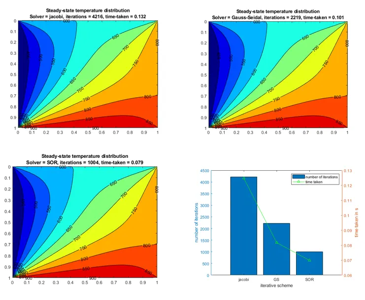
It can be observed from the results displayed above that the three different iterative schemes produce the same end-result. The graph on the bottom right compares the number of iterations taken by each method to converge to the final result. From this graph, it can be inferred that the jacobi requires the highest number of iterations and SOR requires the least iterations. SOR method also depends on the `omega` value. The higher the `omega` value, the lower will be the iterations.
Transient Solution
Explicit
The transient 2D heat equation is represented as
`(dT)/(dt) + (d^2T)/(dx^2) + (d^2T)/(dy^2) = 0` ------------------------------- (4)
The equation (4) is discretized using Forward Euler for time derivative and the CDM for space derivative and the following difference equation is obtained
`T(i,j)^n = T(i,j)^(n-1) – alpha*Deltat*((T(i+1,j)^(n-1) – 2* T(i,j) ^(n-1) + T(i-1,j) ^(n-1))/( Deltax ^2) + (T(i,j+1) ^(n-1) – 2* T(i,j) ^(n-1) + T(i,j-1) ^(n-1))/( Deltay ^2))`
`T_P^n = T_P^(n-1) – alpha*Deltat*((T_R^(n-1) – 2* T_P ^(n-1) + T_L ^(n-1))/( Deltax ^2) + (T_B ^(n-1) – 2* T_P ^(n-1) + T_T ^(n-1))/( Deltay ^2))`
`k_x = (alpha*Deltat)/(Deltax^2) `
`k_y = (alpha*Deltat)/(Deltay^2) `
As it has been established that the explicit schemes are only conditionally stable, this explicit scheme has a criteria, called the CFL criteria to ensure stability of the solution. This criterion is given by
`kx + ky < = 0.5`
% This is the solver for explicit unsteady 2D temp equation
% dT/dt = d^2T/dx^2 + d^2T/dy^2
% centre differencing for 2nd order terms and forward euler for the time

%%
clear all
close all
clc

%% parameters
nx = 40;
ny = 20;
startTime = 0;
endTime = 0.1;
dt = 1e-3;
alpha = 0.5;

%% grids
Lx = 1;
Ly = 2;
x = linspace(0,Ly,nx);
y = linspace(0,Lx,ny);
time = startTime:dt:endTime;
nt = length(time);

dx = x(2) - x(1);
dy = y(2) - y(1);

kx = alpha.*dt./dx.^2
ky = alpha.*dt./dy.^2

%% initialisation
T = zeros(nx,ny,nt);

%% boundary conditions
% top boundary
T(1,:,:) = 600;
% bottom boundary
T(end,:,:) = 900;
% left boundary
T(:,1,:) = 400;
% right boundary
T(:,end,:) = 800;

% corner nodes BC
T(1,1,:) = 0.5*(T(1,2,:) + T(2,1,:));
T(1,end,:) = 0.5*(T(1,end-1,:) + T(2,end,1,:));
T(end,1,:) = 0.5*(T(end-1,1,:) + T(end,2,:));
T(end,end,:) = 0.5*(T(end,end-1,:) + T(end-1,end,:));

%% solving


for t = 2:nt
    for i = 2:nx-1
       for j = 2:ny-1
         T(i,j,t) = T(i,j,t-1) + kx*(T(i+1,j,t-1) - 2*T(i,j,t-1) + T(i-1,j,t-1)) + ky*(T(i,j+1,t-1) - 2*T(i,j,t-1) + T(i,j-1,t-1));

       end

    end


end
fname = 'temperature_unstable2.avi';
plot_sol_transient(T,x,y,time,fname);
In this run, kx and ky were 0.18. Hence the solution was stable.
The script creates the domain with Lx and Ly using linspace command. Then it calculates the kx and ky values and displays it. The user can change the value if needed and proceed with the script. Then the temperature variable is initialised as a 3-dimensional matrix. The first two dimensions are for the space and the third one is for the time. This type of implementation helps in the easy plotting of the results as the same plot function can be used for various purposes. The plot function is available in the appendix.
Then the matrix is initialised with a value of zeros and the appropriate boundary conditions were defined.
The next section deals with the solution of the equation. The outer loop (`t`) deals with the time, the two inner loops (`i` and `j`) deals with the 2D space. Once the solution is completed, the variable T is passed onto the plot function for plotting and creating a video file.
RESULTS:
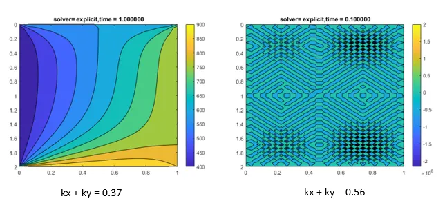
The above picture displays the result obtained from the explicit simulation at the last time-step. The plot on the left shows a stable solution and the one on the right shows an unstable solution. As soon as the CFL condition is violated, the solution becomes unstable quickly as it can be inferred from the time printed on the plot (right). The corresponding video files can be found under the following link
Stable: https://youtu.be/WrPkKCr72Vw
Unstable: https://youtu.be/XnBVD19WYoA
Implicit
In the implicit scheme, the space nodes are taken at the current time step. This implementation produces a linear system of equations which can be solved by the iterative schemes.
`T(i,j)^n = T(i,j)^(n-1) – alpha*Deltat*((T(i+1,j)^(n) – 2* T(i,j) ^(n) + T(i-1,j) ^(n))/( Deltax ^2) + (T(i,j+1) ^(n) – 2* T(i,j) ^(n) + T(i,j-1) ^(n))/( Deltay ^2))`
`T_P^n = T_P^(n-1) – alpha*Deltat*((T_R^(n) – 2* T_P ^(n) + T_L ^(n))/( Deltax ^2) + (T_B ^(n) – 2* T_P ^(n) + T_T ^(n))/( Deltay ^2))`
`T_P^n = 1/(1+2*k_x+2*k_y) * (T_P^(n-1) + k_x * (T_L^(n) + T_R^n) + k_y * (T_T^n + T_B^n))`
`k_x = (alpha*Deltat)/(Deltax^2) `
`k_y = (alpha*Deltat)/(Deltay^2) `
Here also the iterative schemes were implemented as functions similar to the one defined above with the exception of the equation; a different equation is used here.
function [T_solved,err,iter_jacobi] = jacobi_implicit(T,x,y,alpha,tol,dt)

    nx = length(x);
    ny = length(y);

    dx = x(2) - x(1);
    dy = y(2) - y(1);

    kx = alpha.*dt./dx.^2;
    ky = alpha.*dt./dy.^2;

    iter_jacobi = 1;
    err = 9e2;
    Tprev = T;

    while(err > tol)
        Told = T;
        for i = 2:nx-1
            for j = 2:ny-1
                T(i,j) = (1./(1+2*kx+2*ky)).*(Tprev(i,j) + kx*Told(i-1,j) + kx*Told(i+1,j) + ky*Told(i,j-1) + ky*Told(i,j+1));
            end
        end

        err = sum(max(abs(T - Told)));

        iter_jacobi = iter_jacobi + 1;

    end
    T_solved = T;

end
The function takes in the initialised (`T`) variable along with `x` , `y`, `alpha`, `tol` and `dt`. It then follows the same procedure as explained in the section “steady-state solution.” The only difference is that this function is called for every time step and the iteration is performed. So the previous value is stored in variable `Tprev` which will remain constant during the iteration loop. The updated `T` will be returned as `T_solved`. The implementation of the other two solvers are similar to the one described above and can be found in the appendix section.
The main program to execute the implicit solver is shown in the following code snippet.
% this script is to solve the unsteady 2D Temp equation implicitly
% dT/dt = alpha*(d^2T/dx^2 + d^2T/dy^2)


clear all
close all
clc

%% parameters
nx = 20;
ny = 20;
startTime = 0;
endTime = 0.5;
dt = 1e-2;          % time-step size
alpha = 0.5;        % diffusivity co-efficient

tol = 1e-4;         % tolerance for iterative solvers

omega = 1.4;        % extrapolation factor for sor
iterative_solver = "sor";   % solver to be used ["jacobi","gs","sor"]

%% grids
x = linspace(0,1,nx);
y = linspace(0,1,ny);
time = startTime:dt:endTime;
nt = length(time);

%% initialisation
T = zeros(nx,nx,nt);

%% boundary conditions
% top boundary
T(1,:,:) = 600;
% bottom boundary
T(end,:,:) = 900;
% left boundary
T(:,1,:) = 400;
% right boundary
T(:,end,:) = 800;

% corner nodes BC
T(1,1,:) = 0.5*(T(1,2,:) + T(2,1,:));
T(1,end,:) = 0.5*(T(1,end-1,:) + T(2,end,1,:));
T(end,1,:) = 0.5*(T(end-1,1,:) + T(end,2,:));
T(end,end,:) = 0.5*(T(end,end-1,:) + T(end-1,end,:));


%% solving using iterative solvers

switch iterative_solver
    case "jacobi"
        %jacobi
        tic;
        for t = 2:nt
            Tprev = T(:,:,t-1);
            [Tnew,err,iter_jacobi] = jacobi_implicit(Tprev,x,y,alpha,tol,dt);
            T(:,:,t) = Tnew;
            iter = iter_jacobi;

        end
         time_jacobi = toc
         fname = "jacobi_implicit.avi";
         solver="jacobi";

    case "gs"
        %gauss-seidal
        tic;
        for t = 2:nt
            Tprev = T(:,:,t-1);
            [Tnew,err,iter_gs] = GS_implicit(Tprev,x,y,alpha,tol,dt);
            T(:,:,t) = Tnew;
            iter = iter_gs;

        end
        time_gs = toc
        fname = "Gauss_Seidal_implicit.avi";
        solver="Gauss_Seidel";

    case "sor"
        %SOR
        tic;
        for t = 2:nt
            Tprev = T(:,:,t-1);
            [Tnew,err,iter_sor] = SOR_implicit(Tprev,x,y,alpha,omega,tol,dt);
            T(:,:,t) = Tnew;
            iter = iter_sor;

        end
        time_sor = toc
        fname = "SOR_implicit.avi";
        solver="SOR";

    otherwise
        disp("invalid name");
end


%%
plot_sol_transient(T,x,y,time,fname,solver)
The program executes in the same manner as a explicit method except that the iterative solver is called at each time-step. The implicit schemes are unconditionally stable and does not depend on the value of `k_x` or `k_y`. To test this, in this program, these values were used as 1.8. The solution of can be observed in this video.
RESULTS:
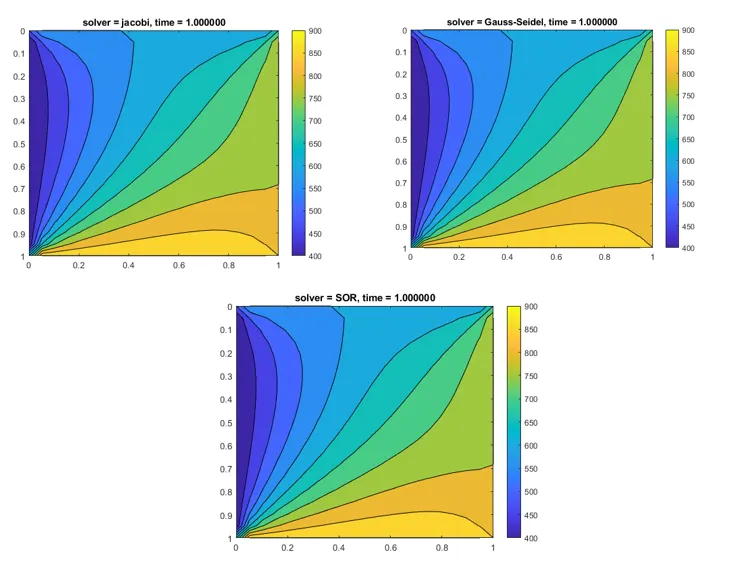
The results from the implicit method are displayed above. All the iterative schemes produce the same final result. Jacobi took the longest time to execute, followed by GS and SOR. As the implicit scheme is unconditionally stable, the value of kx + ky did not play a role in the simulation and the solution remained stable for different values. The corresponding videos can be found under the following links:
Jacobi: https://youtu.be/BPUmetC8ogI
GS: https://youtu.be/Oxbw9piW7zM
SOR: https://youtu.be/Q0XxDhwDwVM
References
- Thermal diffusivity - Wikipedia
- Versteeg, H. K., & Malalasekera, W. (1995). Computational fluid dynamics: the finite volume method. Harlow, England: Longman Scientific & Technical.
- Jacobi Method -- from Wolfram MathWorld
- Gauss-Seidel Method -- from Wolfram MathWorld
- Successive Overrelaxation Method -- from Wolfram MathWorld
Appendix
Implicit_GS_solver
% Gauss-Seidel Method
function [T_solved,err,iter_gs] = GS_implicit(T,x,y,alpha,tol,dt)

    nx = length(x);
    ny = length(y);

    dx = x(2) - x(1);
    dy = y(2) - y(1);

    kx = alpha.*dt./dx.^2;
    ky = alpha.*dt./dy.^2;

    iter_gs = 1;
    err = 9e2;
    Tprev = T;

    while(err > tol)
        Told = T;
        for i = 2:nx-1
            for j = 2:ny-1
                T(i,j) = (1./(1+2*kx+2*ky)).*(Tprev(i,j) + kx*T(i-1,j) + kx*Told(i+1,j) + ky*T(i,j-1) + ky*Told(i,j+1));
            end
        end

        err = sum(max(abs(T - Told)));

        iter_gs = iter_gs + 1;

    end
    T_solved = T;

end
Implicit_SOR_Solver
% SOR Method
function [T_solved,err,iter_sor] = SOR_implicit(T,x,y,alpha,omega,tol,dt)

    nx = length(x);
    ny = length(y);

    dx = x(2) - x(1);
    dy = y(2) - y(1);

    kx = alpha.*dt./dx.^2;
    ky = alpha.*dt./dy.^2;

    iter_sor = 1;
    err = 9e2;
    Tprev = T;

    while(err > tol)
        Told = T;
        for i = 2:nx-1
            for j = 2:ny-1
                T_gs = (1./(1+2*kx+2*ky)).*(Tprev(i,j) + kx*T(i-1,j) + kx*Told(i+1,j) + ky*T(i,j-1) + ky*Told(i,j+1));
                T(i,j) = (1-omega)*Told(i,j) + omega*T_gs;
            end
        end

        err = sum(max(abs(T - Told)));

        iter_sor = iter_sor + 1;

    end
    T_solved = T;

end
Plot Function
function plot_sol_transient(T,x,y,time,fname,solver)
% creating the grid for plotting
[YY,XX] = meshgrid(y,x);
nt = length(time);
% creating video

videoFile = VideoWriter(fname);
videoFile.FrameRate = 30;
open(videoFile)
for t = 1:nt

    contourf(YY,XX,T(:,:,t)); %,'ShowText','on','LabelSpacing',300)
    set(gca,'Ydir','reverse')
    %title(sprintf("Steady-state temperature distribution\nSolver=%s\niterations=%d",solver_name,iter));
    title(sprintf("solver = %s, time = %f",solver,time(t)));
    colorbar
    frame = getframe(gcf);
    writeVideo(videoFile,frame);

end

close(videoFile)
end