Week 5.1 - Mid term project - Solving the steady and unsteady 2D heat conduction problem
GIVEN PROBLEM:
1. Steady state analysis & Transient State Analysis
Solve the 2D heat conduction equation by using the point iterative techniques that were taught in the class. The Boundary conditions for the problem are as follows;
Top Boundary = 600 K
Bottom Boundary = 900 K
Left Boundary = 400 K
Right Boundary = 800 K
You will implement the following methods for solving implicit equations.
1. Jacobi
2. Gauss-seidel
3. Successive over-relaxation
Your absolute error criteria is 1e-4
Make sure to use "INSERT CODE SAMPLE" option to paste the code here. Post screenshots of the plots and use the projects.skill-lync.com page to Publish your findings.
2. You will write code for both implicit and explicit schemes (This is for the Transient Analysis only)
3. Write a detailed explanation for your results, plots or codes without explanation will awarded zero marks.
Theory:
conduction is a mode of heat transfer generally takes place in solids due to temperature difference associated with
free electron and lattice vibration. The equation is given by:
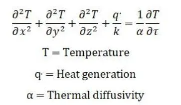
Thermal diffusivity is a property of a material defined as thermal conductivity and thermal capacity
since it a 2D heat conduction problem and there is no internal heat generation,so the equation is parabolic.
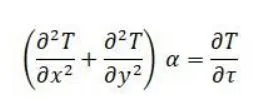
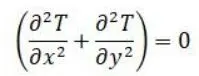
For steady state time derivative is not constant,so the equation is eliptical
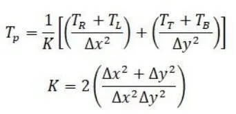
To obtain numeric solution of 2D steady and unsteady heat conduction equation difference equations are
steady state 2-D heat conduction:
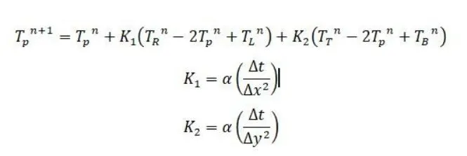
Transient 2-D heat conduction equation(explicit):
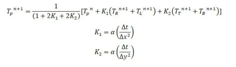
Transient 2-D heat conduction (implicit):
CODE FOR STEADY-STATE EQUATION:
FUNCTION CODE:
jacobi
function out=jacobi(T,T_old,i,j)
nx=10;
ny=10;
x=linspace(0,1,nx);
dx=x(2)-x(1);
y=linspace(0,1,ny);
dy=y(2)-y(1);
k=(2*dx^2+2*dy^2)/(dx^2*dy^2);
term1=(T_old(i+1,j)+T_old(i-1,j))/dx^2;
term2=(T_old(i,j+1)+T_old(i,j-1))/dy^2;
out=(term1+term2)/k;
gauss
function out=GS(T,T_old,i,j)
nx=10;
ny=10;
x=linspace(0,1,nx);
dx=x(2)-x(1);
y=linspace(0,1,ny);
dy=y(2)-y(1);
k=(2*dx^2+2*dy^2)/(dx^2*dy^2);
term1=(T_old(i+1,j)+T(i-1,j))/dx^2;
term2=(T_old(i,j+1)+T(i,j-1))/dy^2;
out=(term1+term2)/k;
SOR
function out=sor(T,T_old,i,j,omega)
nx=10;
ny=10;
x=linspace(0,1,nx);
dx=x(2)-x(1);
y=linspace(0,1,ny);
dy=y(2)-y(1);
k=(2*dx^2+2*dy^2)/(dx^2*dy^2);
term1=(T_old(i+1,j)+T(i-1,j))/dx^2;
term2=(T_old(i,j+1)+T(i,j-1))/dy^2;
out=((1-omega)*T_old(i,j))+(omega*((term1+term2)/k));
MAIN CODE
clear
close all
clc
%inputs
%grid points along x and y axis
nx=10;
ny=10;
x=linspace(0,1,nx);
dx=x(2)-x(1);
y=linspace(0,1,ny);
dy=y(2)-y(1);
%initial temperature values for all nodes
T=300*ones(nx,ny);
%initial boundary condition at the top and botttom
T(1,:)=600;
T(end,:)=900;
%initial boundary condition at the left and right
T(:,1)=400;
T(:,end)=800;
%copy temperature to compute
T_old=T;
T_prev=T;
% initializing error value
error=9e9;
tolerance=1e-4;
omega=1.2;
for iterative_solver=1:3
if iterative_solver==1
iter=1;
while error>tolerance
for i=2:nx-1
for j=2:ny-1
T(i,j)=jacobi(T,T_old,i,j);
end
end
error=max(max(abs(T_old-T)));
%updating value of T
T_old=T;
figure(1)
[u,v]=meshgrid(x,y);
[c,h]= contourf(u,v,T);
colorbar
colormap("jet")
clabel(c,h)
set(gca,'ydir','reverse')
iter_method=sprintf('jacobi iteration is:%d',iter);
title(iter_method);
iter=iter+1;
end
elseif iterative_solver==2
T_old=T_prev;
iter1=1;
while error>tolerance
for i=2:nx-1
for j=2:ny-1
T(i,j)=GS(T,T_old,i,j);
end
end
error=max(max(abs(T_old-T)));
%updating value of T
T_old=T;
figure(2)
[u,v]=meshgrid(x,y);
[c,h]=contourf(u,v,T);
colorbar
colormap("jet")
set(gca,'ydir','reverse')
clabel(c,h)
iter_method=sprintf('GS iteration is:%d',iter1);
title(iter_method);
iter1=iter1+1;
end
elseif iterative_solver==3
iter2=1;
T_old=T_prev;
while error>tolerance
for i=2:nx-1
for j=2:ny-1
T(i,j)=sor(T,T_old,i,j,omega);
end
end
error=max(max(abs(T_old-T)));
%updating value of T
T_old=T;
figure(3)
[u,v]=meshgrid(x,y);
[c,h]= contourf(u,v,T);
colorbar
colormap("jet")
set(gca,'ydir','reverse')
clabel(c,h);
iter_method=sprintf('sor iteration is:%d',iter2);
title(iter_method);
iter2=iter2+1;
end
end
error=9e9;
T_old=T;
end
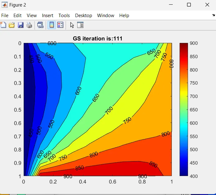
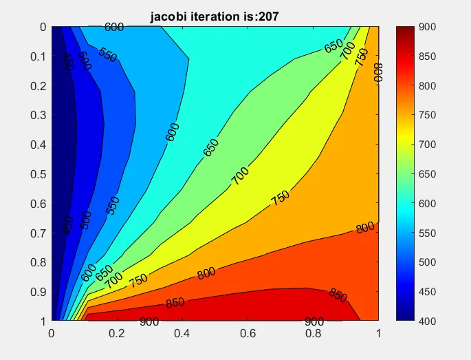
OUTPUT
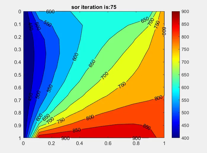
EXPLANATION:
1.First of all we take n number of nodes along x and y axis as nx and ny . Distance between two nodes along x and y axis are
dx and dy. we take temperature at each point is 300k and then take boundary conditions like top and bottom temperature are
600k and 900k and left and right are 400k and 800k.
2.We take two copy of initial conditions of temperature, T as T_old and T_prev.Take a random value of error is 9e^9 and tolerance is 1e^-4 so as error should be greater than tolrance as we have to reduce error value up to tolerance so as to achieve perfection from imperfection.Also taking the value of omega as 1.2 , if we incraese omega more so we mayface more iteration thus incorporating wrong result.
3.we have to adopt a iterative_solver (a variable)to check this method for three formulas as jacobi,gauss-seidal and sor.
Vary the iterative_solver from 1 to 3 and check each formula by if-else condition.
4.In previous its discussed that we should decrease error upto level of tolerance so we adopt a while loop where error>tolerance.Then as its a 2D problem so we have to take two for loop as i & j and vary it from 2 to (n-1) as boundary
conditions are known.
5.After for loops we are updating error value as maximum difference of T_old and newly derived T. we have to update
T_old=T as the newly derived T will be T_old in the loop for the next iteration. In each loop we have to take iteration value
before while loop and increment it by "itreration=iteration+1" before while loop finishes.These all are done at each iterative_solver.
6.We are taking x,y command as 2d form by meshgrid command and plot it by contourf command.We are taking a column like entity to show how the colors are distributed by colorbar command , we can make different types of shades of color by
colormap command.we are pointing sizes of each plot by clabel command.
7.After declaring title_method by sprintf we are taking it as title of the plot.
8.At iterative_solver=2 before while loop we are taking T_old=T_prev, as the T_old should be first value before iterative_solver=1 ,so that it can start iteration from the first T_old value otherwise T_old value will be taken after it had been
iterated at the end of the iterative_solver=1. same is done for the iterative_solver=3.
CODE FOR NON-STEADY STATE EQUATION:
close all
clear all
clc
% Transient State Heat Conduction
% dt^2/dT^2 + aplha(d^2T/dx^2 + d^2T/dy^2)=0
nx = 10;
ny = 10;
T = 450*ones(nx,ny);
TL = 400;
TR = 800;
TT = 600;
TB = 900;
% Boundary Conditions
T(:,1) = TL;
T(:,ny) = TR;
T(1,:) = TT;
T(nx,:) = TB;
% Edge Refinement
T(1,1) = (T(1,2)+T(2,1))/2;
T(1,ny) = (T(1,(ny-1))+T(2,ny))/2;
T(nx,1) = (T((nx-1),1)+T(nx,2))/2;
T(nx,ny) = (T(nx,(ny-1))+T((nx-1),ny))/2;
% Inputs
% Time Step
dt = 1e-2;
% Grid Spacing
dx = 1.3e-2;
dy = 1.3e-2;
% Thermal Diffusibility
alpha = 0.004;
k1 = alpha*dt/dx^2;
k2 = alpha*dt/dy^2;
cfl = k1 + k2
% Copy of previous result %
T_previous = T;
conv = 9e9;
tol = 1e-4;
time_iteration = 0;
% Time Looping %
while (conv > tol)
for i = 2:nx-1
for j = 2:ny-1
T(i,j) = (1-2*k1-2*k2)*T_previous(i,j) + k1*(T_previous(i+1,j)+ T_previous(i-1,j)) +k2*(T_previous(i,j+1) + T_previous(i,j-1));
end
end
conv = max(max(abs(T-T_previous)));
T_previous = T;
time_iteration = time_iteration +1;
figure(1)
contourf(flipud(T),'ShowText','ON')
title(sprintf('Transient Explicit Iteration = %d',time_iteration));
pause(0.003)
end
colorbar
% Program for Transient-State 2D Heat Conduction using Explicit Method %
close all
clear all
clc
% Transient State Heat Conduction
% dt^2/dT^2 + aplha(d^2T/dx^2 + d^2T/dy^2) = 0)
nx = 10;
ny = 10;
T = 450*ones(nx,ny);
TL = 400;
TR = 800;
TT = 600;
TB = 900;
% Boundary Conditions
T(:,1) = TL;
T(:,ny) = TR;
T(1,:) = TT;
T(nx,:) = TB;
% Edge Refinement
T(1,1) = (T(1,2)+T(2,1))/2;
T(1,ny) = (T(1,(ny-1))+T(2,ny))/2;
T(nx,1) = (T((nx-1),1)+T(nx,2))/2;
T(nx,ny) = (T(nx,(ny-1))+T((nx-1),ny))/2;
% Inputs from Assesment %
% Time Step for iterations
dt = 1e-2;
% Grid Spacing for accurate results
dx = 1e-2;
dy = 1e-2;
% Thermal Diffusibility constant
alpha = 1.5;
k1 = alpha*dt/dx^2
k2 = alpha*dt/dy^2
% Saving a Copy
Told = T;
T_initial = T;
T_prev = T;
error = 9e9;
conv = 9e9;
tol = 1e-4;
% Iteration Solvers - Jacobi || GS || SOR
% 1- Jacobi Method
jacobi_iteration = 0;
jacobi_time_iterations = 0;
% Time Loop for iterations %
while (conv > tol)
% Space Loop
while (error > tol)
for i = 2:nx-1
for j = 2:ny-1
T(i,j) = (1+2*k1+2*k2)^-1 *(T_prev(i,j)+ k1*(Told(i+1,j)+ Told(i-1,j)) +k2*(Told(i,j+1) + Told(i,j-1)));
end
end
error = max(max(abs(T-Told)));
Told = T;
jacobi_iteration = jacobi_iteration +1;
figure(1)
contourf(flipud(T),'ShowText','ON')
title(sprintf('Transient Implicit Jacobi Iteration = %d \n Time Iteration = %d',jacobi_iteration,jacobi_time_iterations));
pause(0.003)
end
conv = max(max(abs(T-T_prev)));
T_prev = T;
jacobi_time_iterations = jacobi_time_iterations +1;
error = 9e9;
end
colorbar
% Reinitialising the old values %
T = T_initial;
Told = T;
T_prev = T;
error = 9e9;
conv = 9e9;
% 2 ------ Gauss Seidel Method %
gs_iteration = 0;
gs_time_iteration =0;
% Time Loop
while (conv > tol)
% Space Loop
while (error > tol)
for i = 2:nx-1
for j = 2:ny-1
T(i,j) = (1+2*k1+2*k2)^-1 *(T_prev(i,j)+ k1*(Told(i+1,j)+ T(i-1,j)) +k2*(Told(i,j+1) + T(i,j-1)));
end
end
error = max(max(abs(T-Told)));
Told = T;
gs_iteration = gs_iteration +1;
figure(2)
contourf(flipud(T),'ShowText','ON')
title(sprintf('Transient Implicit Gauss Siedel Iteration = %d \n Time Iteration = %d',gs_iteration,gs_time_iteration));
pause(0.003)
end
conv = max(max(abs(T-T_prev)));
T_prev = T;
gs_time_iteration = gs_time_iteration +1;
error = 9e9;
end
colorbar
% Reinitialising
T = T_initial;
Told = T;
T_prev = T;
error = 9e9;
conv = 9e9;
% 3- Successive over-relaxation (SOR)
sor_iteration = 0;
sor_time_iteration = 0;
omega = 1.5;
% Time Loop
while (conv > tol)
% Space Loop
while (error > tol)
for i = 2:nx-1
for j = 2:ny-1
TGS(i,j) = (1+2*k1+2*k2)^-1 *(T_prev(i,j)+ k1*(Told(i+1,j)+ T(i-1,j)) +k2*(Told(i,j+1) + T(i,j-1)));
T(i,j) = (1-omega)*Told(i,j) + omega*TGS(i,j);
end
end
error = max(max(abs(T-Told)));
Told = T;
sor_iteration = sor_iteration +1;
figure(3)
contourf(flipud(T),'ShowText','ON')
title(sprintf('Transient Implicit Successive over-relaxation Iteration = %d \n Time Iteration = %d',sor_iteration,sor_time_iteration));
pause(0.003)
end
conv = max(max(abs(T-T_prev)));
T_prev = T;
sor_time_iteration = sor_time_iteration +1;
error = 9e9;
end
colorbar
output
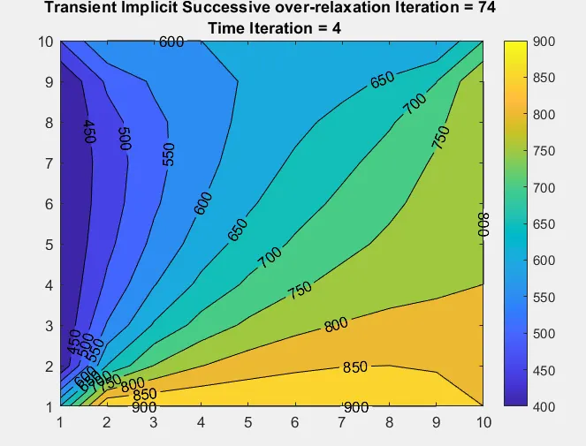
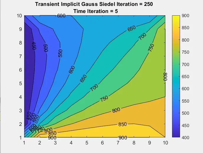
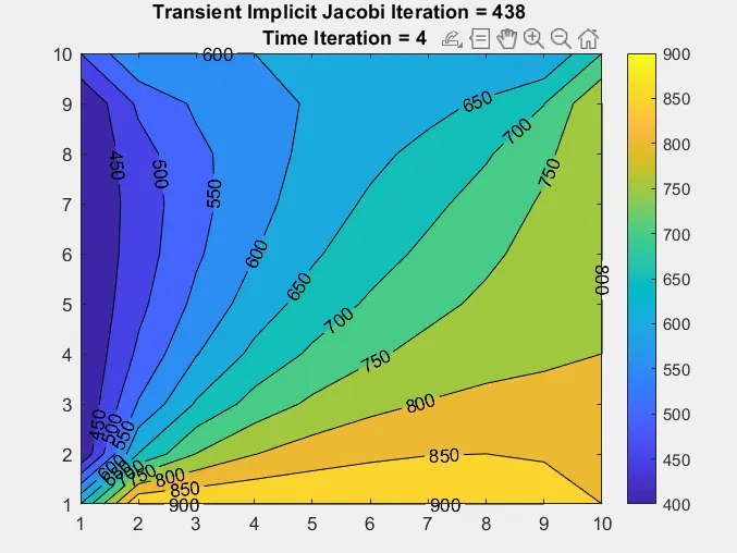
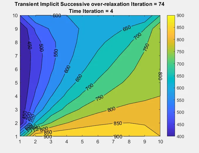
CONCLUSION:
1.We can conclude that for steady or unsteady sor is faster than gauss and then gauss is faster than jacobi.
2.Then for unsteady-state explicit method is much faster than implicit.