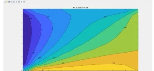
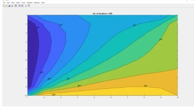
Week 5.1 - Mid term project - Solving the steady and unsteady 2D heat conduction problem
AIM– SOLVING THE STEADY AND UNSTEADY 2D HEAT CONDUCTION PROBLEM
Steady-State Analysis and Transient State Analysis
OBJECTIVE
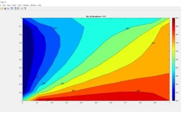
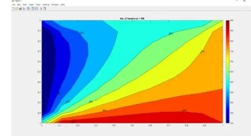
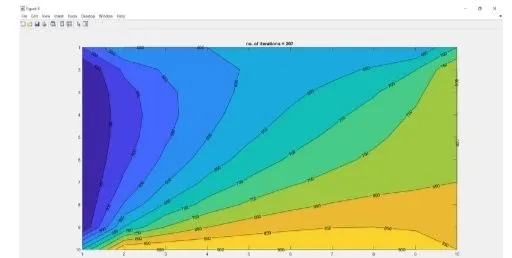
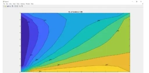
Solve the 2D heat conduction equation by using the point iterative techniques.
Implement the following methods for solving implicit equations;
Jacobi
Gauss – seidel
Successive over-relaxation
Write the transient analysis code for both implicit and explicit schemes.
GIVEN
The Boundary conditions for the problem are as follows;
Top Boundary = 600 k
Bottom Boundary = 900k
Left Boundary = 400 k
Right Boundary = 800 k
Absolute error criteria = 1e - 4
SOLUTION
Thermal Conduction
Heat is transferred by conduction when adjacent atoms or molecules collide, or as several electrons move backwards and forwards from atom to atom in a diagnosed way so as not to form a macroscopic electric current, or as photons collide and scatter. Conduction is the most significant means of heat transfer within a solid or between solid objects in thermal contact.
The 2D temperature heat equation is a partial differential equation.
dTdt–α⋅(∂2T∂x2+∂T2∂y2)=0">dTdt–α⋅(d2Tdx2+dT2dy2)=0
Here, alpha is a positive coefficient called the thermal diffusivity of the medium.
Steady-State Conduction
Steady-state conduction is the form of conduction that happens when the temperature difference driving the conduction is constant so that the spatial distribution of temperatures in the conducting object does not change any further. Thus, all partial derivatives of temperature concerning space may either be zero or have nonzero values, but all derivatives of temperature at any point concerning time are uniformly zero. In steady-state conduction, the amount of heat entering any region of an object is equal to the amount of heat coming out, i.e.
∂2T∂x2+∂T2∂y2=0">d2Tdx2+dT2dy2=0
Transient Conduction
During any period in which temperatures change in time at any place within an object, the mode of thermal energy flow is termed transient conduction. Another term is "non-steady-state" conduction, referring to the time-dependence of temperature fields in an object. Non-steady-state situations appear after an imposed change in temperature at a boundary of an object. The formula for the 2D transient heat conduction equation is:
∂T∂t=(α)⋅(∂2T∂x2+∂2T∂y2)">dTdt=(α)⋅(d2Tdx2+d2Tdy2)
EXPLICIT AND IMPLICIT METHODS are approaches used in numerical analysis for obtaining numerical approximations to the solutions of time-dependent ordinary and partial differential equations, as is required in computer simulations of physical processes.
Iterative Method
In computational mathematics, an iterative method is a mathematical procedure that uses an initial value to generate a sequence of improving approximate solutions for a class of problems, in which the n-th approximation is derived from the previous ones. A specific implementation of an iterative method, including the termination criteria, is an algorithm of the iterative method. An iterative method is called convergent if the corresponding sequence converges for given initial approximations.
Iterative Solver
- Jacobi iterative solver
The Jacobi method is an iterative algorithm for determining the solutions of a strictly diagonally dominant system of linear equations. Each diagonal element is solved for, and an approximate value is plugged in. The process is then iterated until it converges.
- Gauss-Seidel iterative solver
The Gauss-seidel method, or the method of successive displacement, is an iterative method used to solve a system of linear equations similar to the Jacobi method. The temperature at n+1 iterations uses values of n+1 iterations that have already been computed. In this path, old approximated values are overwritten with new approximate values for the iterations performed. Unlike Jacobi, Gauss-Seidel requires one storage vector which can be overwritten with each computation. This helps the solution to converge faster than the Jacobi method.
- Successive over-relaxation iterative solver
SOR is a variant of the Gauss-Seidel method for solving a linear system of equations, resulting in faster convergence. This exploration takes the form of a weighted average between the previous iterate and the computed Gauss-Seidel iterate successively for each component.
Formula: Tt+1 = Tts . (1-w) + w. T(GS)n+1 or T(Jacobi)n+1
Here, w is the relaxation factor.
Range: 0 < w < 2
0 < w < 1 (Under-Relaxed state)
This condition is used when the temperature gradient is high and due to this condition, the time step does not overshoot and helps to converge at a faster rate.
1 < w < 2 (Over-Relaxed state)
This condition is used when the temperature gradient is low and due to this condition more significant time steps are used to obtain the steady-state, i.e. for the values to converge at a faster rate.
Nomenclature
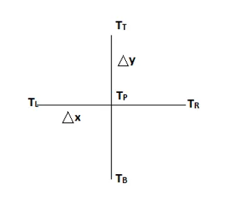
TP = Ti, j
TL = Ti-1, j (Left boundary)
TR = Ti+1, j (Right boundary)
TT = Ti, j+1 (Top boundary)
TB = Ti, j-1 (Bottom boundary)
Equations used
2D heat conduction equation:
dTdt–α⋅(∂2T∂x2+∂T2∂y2)=0">dTdt–α⋅(d2Tdx2+dT2dy2)=0
In discrete form:
Ti+1,j^n-2Ti,j^n+Ti-1,j^n/dx2+Ti,j+1-2Ti,j^n+Ti,j-1^n/dy2=1/<Ti,j^n+1-Ti,j^n/dt
Here,
n represents the current time step and n+1 represents the next time step.
i, i+1 are the neighbouring points in the x-direction.
j, j+1 are the neighbouring points in the y-direction.
∠x">∠x is grid spacing in the x-direction.
∠y">∠y
is grid spacing in the y-direction.
The time derivative term is hyperbolic in nature which is to be discretised using a forward differencing scheme and the space derivatives are elliptical in nature which is to be discretised using a central differencing scheme.
Steady State 2D Heat Conduction Equation
∂2T∂x2+∂T2∂y2=0">d2Tdx2+dT2dy2=0
>Steady State Discretization
(TL – 2.TP + TR)/ ∠x2">∠x2
+ (TT – 2.TP + TB)/ ∠y2">∠y2
= 0;
- TL-2.TP+TR/dx2+TT-2.TP+TB/dy2=0
- Therefore,
TP= K1 (TT + TR) + K2 (TT + TB)
Where,
K1 = ∠y22.(∠x2+∠y2)">∠y22.(∠x2+∠y2)
and K2 = ∠x22.(∠x2+∠y2)">∠x22.(∠x2+∠y2)
>Using iterative solvers for solving the conduction equation steady state:
Jacobi iterative solver
(TP)n+1 = K1 (TL + TR)n + K2 (TT + TB)n
Gauss-Seidel iterative solver
(TB)n+1 = K1 (TL + TR)n+1 + K2 (TT + TB)n+1
Successive over relaxation iterative solver
(TP)n+1 = (TP)n.(1-w) + w.( K1(TL +TR)n+1 + K2(TT+ TB)n+1)>
Transient State
∂T∂t=α⋅(∂2T∂x2+∂2T∂y2)">dTdt=α⋅(d2Tdx2+d2Tdy2)
>Unsteady-State Discretization
>Solving Explicitly
(TP)n+1 = (1 - 2.K1 – 2.K2).(TP)n + K1(TL + TR)n + K2(TT + TB)n
Here,
K1 = α.∠t∠x2">α.∠t∠x2
K2 = α.∠t∠y2">α.∠t∠y2
>Stability Criteria
K1 + K2 ≤">≤
0.5
>Solving Implicitly
(1 - 2.K1 – 2.K2).(TP)n+1 = (TP)n + K1 (TL + TR)n+1 + K2 (TT + TB)n+1
Here,
K1 = α.∠t∠x2">α.∠t∠x2
K2 = α.∠t∠y2">α.∠t∠y2
Jacobi iterative solver
(TP)n+1 = ((TP)n + K1 ((TL)n + (TR)n) + K2 ((TT)n + (TB)n) / (1 - 2.K1 – 2.K2)
Gauss-Seidel iterative solver
(TP)n+1 = ((TP)n + K1 ((TL)n+1 + (TR)n) + K2 ((TT)n + (TB)n+1) / (1 - 2.K1 – 2.K2)
Successive over-relaxation iterative solver
(TP)n+1 = (TP)n . (1 - w) + w. [((TP)n + K1 ((TL)n+1 + (TR)n) + K2 ((TT)n + (TB)n+1) / (1 - 2.K1 – 2.K2)]
ASSUMPTIONS
>Consider computation area as a square.
>nx = ny; i.e., the number of nodes in the x-direction is equal to the number of nodes in the y-direction.
>nx = ny = 10
>Apart from the boundary conditions, the inner nodes have an initial temperature value of 300K.
Boundary Conditions
>Top Boundary = 600 k
>Bottom Boundary = 900k
>Left Boundary = 400 k
>Right Boundary = 800 k
code to study the STEADYand UMSTEADY state for 2D heat conduction
MATLAB CODE
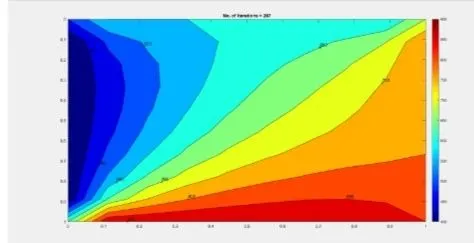
Gauss-Seidel iterative method for steady-state