Week 5.1 - Mid term project - Solving the steady and unsteady 2D heat conduction problem
The following Project is to solve The Heat Conduction Equation, both steady and unsteady state, using the Point Iterative techniques. The Boundary conditions are given as follows:
Top Boundary=600K
Bottom Boundary=900K
Left Boundary=400K
Right Boundary=800K
The error criterion e=1e-4
Solution:
The general form of Heat conduction equation(in 2-Dimensions) is:
`(dT)/dt= alpha((d^2T)/dx^2+(d^2T)/dy^2)`
This equation is for Transient or Unsteady conditions, where Temperature varies with respect to time for a given fluid flow.
For steady state condition, the rate of change of Temperature with change in time becomes negligible, hence in from the above equation `(dT)/dt` equals 0(in Steady state condition).
Hence, the Heat conduction equation for Steady state becomes:
`alpha((d^2T)/dx^2+(d^2T)/dy^2)=0`
Now if we discretize the above Steady State heat conduction equation using Central Difference scheme(since the Differential Equation is Elliptic in Nature), we get:
`(d^2T)/dx^2=(T(i-1,j)-2.T(i,j)+T(i+1,j))/(trianglex^2)`
and
`(d^2T)/dy^2=(T(i,j-1)-2.T(i,j)+T(i,j+1))/(triangley^2)`
Now we assume nx=ny(square mesh), hence `trianglex^2=triangley^2`. Then the above 2equations becomes:
`T(i,j)=1/4(T(i-1,j)+T(i+1,j)+T(i,j-1)+T(i,j+1))`
Similarly, for Transient State Heat conduction equation:
`(Tp^(n+1)-Tp)/(trianglet)= alpha((Tl-2.Tp+Tr)/(trianglex^2)+(Tt-2.Tp+Tb)/(triangley^2))`
where: Tp= temperature at point of consideration. Tt, Tb, Tl and Tr are top. bottom, left and right point temperatures to Tp. If this equation is calculated at n time step, it becomes Explicit form and if it is calculated at n+1 time step it becomes Implicit form.
Now ,on solving the above equation:
`Tp^(n+1)= Tp^n+k1(Tl-2.Tp+Tr)^n+k2(Tt-2.Tp+Tb)^n`-Explicit form
`Tp^(n+1)=1/(1+2k1+2k2)(Tp^n+k1(Tl+Tr)^(n+1)+k2(Tt+Tb)^(n+1))`
where
`k1= (alphatriangleT)/(trianglex^2)` and `k2=(alphatriangleT)/(triangley^2)`
k1 and k2 are the CFL numbers. CLF should be `<=`0.5 for stability of the equation.
Following are the Matlab Codes(along with required explainations) and the outputs for different iterative schemes, using which Heat conduction equation is solved:
1.STEADY STATE JACOBI METHOD:
CODE:
clear all;
close all;
clc;

%INPUTS
L=1;                  %Length of the Domain
nx=30;                %number of grid points
ny=nx;

x=linspace(0,L,nx);
y=linspace(0,L,ny);
dx=x(2)-x(1);
dy=y(2)-y(1);

error=10000;
tol=1e-4;              %tolerance value

%Given Temperatures at boundary
T_L=400;
T_T=600;
T_R=800;
T_B=900;
T=ones(nx,ny);
T(2:ny-1,1)= T_L;
T(2:ny-1,nx)= T_R;
T(1,2:nx-1)= T_T;
T(nx,2:ny-1)= T_B;

%Temperature at edges of the grid
T(1,1)= (T_T+T_L)/2;
T(nx,ny)= (T_R+T_B)/2;
T(1,ny)= (T_T+T_R)/2;
T(nx,1)= (T_L+T_B)/2;

[X,Y]= meshgrid(x,y);
Told=T;
tic
jacobi_iter=1;
while(error>tol)
  for (i=2:nx-1)
    for (j=2:ny-1)
      T(i,j)= 0.25*(Told(i+1,j)+Told(i-1,j)+Told(i,j-1)+Told(i,j+1));
    end
  end
  error=max(max(abs(Told-T)));
  Told=T;
  jacobi_iter=jacobi_iter+1;
end
F=toc;

figure(i)
[M,N]=contourf(x,y,T);
clabel(M,N);
colormap(jet);
colorbar;
title_text=sprintf('Steady State (Jacobi) Iteration no.%d,Total time= %fs',jacobi_iter,F);
title(title_text);
xlabel('Length');
ylabel('Height');
set(gca,'Ydir','reverse');
fprintf('Steady State Jacobi Iteration no.%d\n',jacobi_iter);
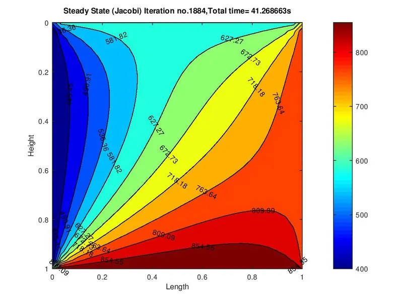
OUTPUT:
2. STEADY STATE GAUSS SEIDEL METHOD:
CODE:
clear all;
close all;
clc;

%INPUTS
L=1;                  %Length of the Domain
nx=30;                %number of grid points
ny=nx;

x=linspace(0,L,nx);
y=linspace(0,L,ny);
dx=x(2)-x(1);
dy=y(2)-y(1);

error=10000;
tol=1e-4;              %tolerance value

%Given Temperatures at boundary
T_L=400;
T_T=600;
T_R=800;
T_B=900;
T=ones(nx,ny);
T(2:ny-1,1)= T_L;
T(2:ny-1,nx)= T_R;
T(1,2:nx-1)= T_T;
T(nx,2:ny-1)= T_B;

%Temperature at edges of the grid
T(1,1)= (T_T+T_L)/2;
T(nx,ny)= (T_R+T_B)/2;
T(1,ny)= (T_T+T_R)/2;
T(nx,1)= (T_L+T_B)/2;

[X,Y]= meshgrid(x,y);
Told=T;
tic
GS_iter=1;
while(error>tol)
  for (i=2:nx-1)
    for (j=2:ny-1)
      T(i,j)= 0.25*(Told(i+1,j)+T(i-1,j)+T(i,j-1)+Told(i,j+1));
    end
  end
  error=max(max(abs(Told-T)));
  Told=T;
  GS_iter=GS_iter+1;
end
F=toc;

figure(i)
[M,N]=contourf(x,y,T);
clabel(M,N);
colormap(jet);
colorbar;
title_text=sprintf('Steady State (G-S) Iteration no.%d,Total time= %fs',GS_iter,F);
title(title_text);
xlabel('Length');
ylabel('Height');
set(gca,'Ydir','reverse');
fprintf('Steady State G-S Iteration no.%d\n',GS_iter);
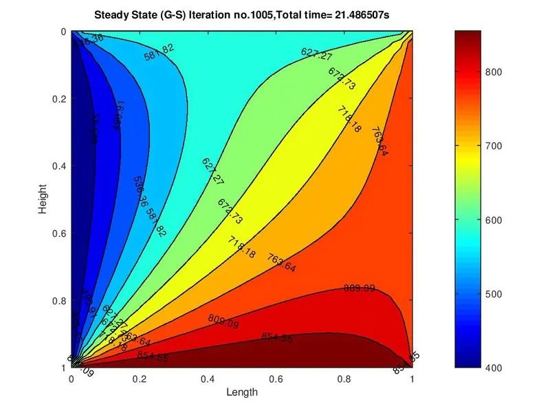
OUTPUT:
3. STEADY STATE SUCCESSIVE OVER-RELAXATION METHOD:
CODE:
clear all;
close all;
clc;

%INPUTS
L=1;                  %Length of the Domain
nx=30;                %number of grid points
ny=nx;

x=linspace(0,L,nx);
y=linspace(0,L,ny);
dx=x(2)-x(1);
dy=y(2)-y(1);

error=10000;
tol=1e-4;              %tolerance value
alpha= 1.8;                %Relaxation Factor for SOR Method

%Given Temperatures at boundary
T_L=400;
T_T=600;
T_R=800;
T_B=900;
T=ones(nx,ny);
T(2:ny-1,1)= T_L;
T(2:ny-1,nx)= T_R;
T(1,2:nx-1)= T_T;
T(nx,2:ny-1)= T_B;

%Temperature at edges of the grid
T(1,1)= (T_T+T_L)/2;
T(nx,ny)= (T_R+T_B)/2;
T(1,ny)= (T_T+T_R)/2;
T(nx,1)= (T_L+T_B)/2;

[X,Y]= meshgrid(x,y);
Told=T;
tic
SOR_iter=1;
while(error>tol)
  for (i=2:nx-1)
    for (j=2:ny-1)
      T(i,j)= (1-alpha)*Told(i,j)+(alpha*0.25*(Told(i+1,j)+T(i-1,j)+T(i,j-1)+Told(i,j+1)));
    end
  end
  error=max(max(abs(Told-T)));
  Told=T;
  SOR_iter=SOR_iter+1;
end
F=toc;

figure(i)
[M,N]=contourf(x,y,T);
clabel(M,N);
colormap(jet);
colorbar;
title_text=sprintf('Steady State (SOR) Iteration no.%d,Total time= %fs',SOR_iter,F);
title(title_text);
xlabel('Length');
ylabel('Height');
set(gca,'Ydir','reverse');
fprintf('Steady State SOR Iteration no.%d\n',SOR_iter);
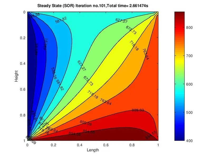
OUTPUT:
4. TRANSIENT EXPLICIT SCHEME:
CODE:
clear all;
close all;
clc;

%INPUTS
L=1;                  %Length of the Domain
nx=10;                %number of grid points
ny=nx;
q=1.4;

x=linspace(0,L,nx);
y=linspace(0,L,ny);
dx=x(2)-x(1);
dy=y(2)-y(1);

error=10000;
tol=1e-4;              %tolerance value
dt=0.001;

%Given Temperatures at boundary
T_L=400;
T_T=600;
T_R=800;
T_B=900;
T=ones(nx,ny);
T(2:ny-1,1)= T_L;
T(2:ny-1,nx)= T_R;
T(1,2:nx-1)= T_T;
T(nx,2:ny-1)= T_B;

%Temperature at edges of the grid
T(1,1)= (T_T+T_L)/2;
T(nx,ny)= (T_R+T_B)/2;
T(1,ny)= (T_T+T_R)/2;
T(nx,1)= (T_L+T_B)/2;

[X,Y]= meshgrid(x,y);
Told=T;
Tprev=T;

k1=(q*dt)/dx^2;
k2=(q*dt)/dy^2;

tr_explicit=1;
tic
for nt=1:1000
  while(error>tol)
    for i=2:nx-1
      for j=2:ny-1
        T(i,j)= Told(i,j)+ (k1*(Told(i+1,j)-(2*Told(i,j))+Told(i-1,j)))+(k2*(Told(i,j+1)-(2*Told(i,j))+Told(i,j-1)));
      endfor
    endfor
    error=max(max(abs(Told-T)));
    Told=T;
    tr_explicit=tr_explicit+1;
    end
    endfor
F=toc;

%%plot
figure(i)
[M,N]= contourf(x,y,T);
clabel(M,N);
colormap(jet);
colorbar;
title_text=sprintf('Transcient iteration number through explicit=%d, Total Time= %fs',tr_explicit,F);
title(title_text);
xlabel('X-axis');
ylabel('Y-axis');
set(gca,'Ydir','reverse');
fprintf('Number of iteration in Transient(Explicit)=%d\n',tr_explicit);
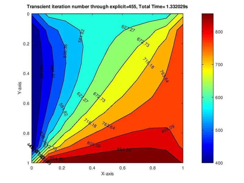
OUTPUT:
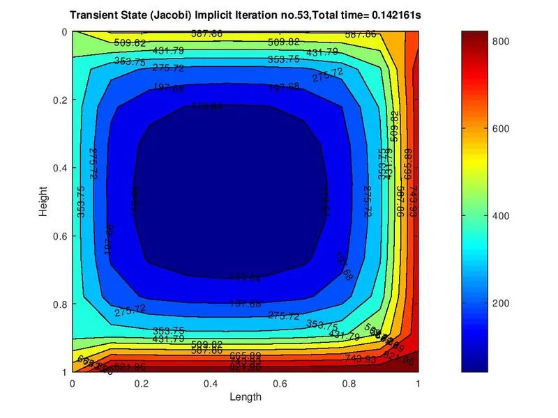
5. TRANSIENT IMPLICIT SCHEME USING JACOBI METHOD:
CODE:
clear all;
close all;
clc;

%INPUTS
L=1;                  %Length of the Domain
b=1;
nx=10;                %number of grid points
ny=nx;

x=linspace(0,L,nx);
y=linspace(0,L,ny);
dx=x(2)-x(1);
dy=y(2)-y(1);
error=10000;
tol=1e-4;              %tolerance value
q=1.4;
dt=0.01;

%Given Temperatures at boundary
T_L=400;
T_T=600;
T_R=800;
T_B=900;
T=ones(nx,ny);
T(2:ny-1,1)= T_L;
T(2:ny-1,nx)= T_R;
T(1,2:nx-1)= T_T;
T(nx,2:ny-1)= T_B;

%Temperature at edges of the grid
T(1,1)= (T_T+T_L)/2;
T(nx,ny)= (T_R+T_B)/2;
T(1,ny)= (T_T+T_R)/2;
T(nx,1)= (T_L+T_B)/2;

k1=q*((dt)/(dx^2));
k2=q*((dt)/(dy^2));
[X,Y]= meshgrid(x,y);
Told=T;
Tprev=Told;

term1=(((2*k1)+(2*k2)+1)^(-1));
term2=k1*term1;
term3=k2*term1;

tic
jacobi_iter=1;
for nt=1:1400
while(error>tol)
  for (i=2:nx-1)
    for (j=2:ny-1)
      T(i,j)= (term1*Tprev(i,j))+(term2*(Told(i-1,j)+Told(i+1,j)))+(term3*(Told(i,j-1)+Told(i,j+1)));
    end
  end
  error=max(max(abs(Told-T)));
  Told=T;
  jacobi_iter=jacobi_iter+1;
end
Tprev=T;
endfor
F=toc;

figure(i)
[M,N]=contourf(x,y,T);
clabel(M,N);
colormap(jet);
colorbar;
title_text=sprintf('Transient State (Jacobi) Implicit Iteration no.%d,Total time= %fs',jacobi_iter,F);
title(title_text);
xlabel('Length');
ylabel('Height');
set(gca,'Ydir','reverse');
fprintf('Transient State Jacobi Iteration no.%d\n',jacobi_iter);
OUTPUT:
6. TRANSIENT IMPLICIT SCHEME USING GAUSS SEIDEL METHOD:
CODE:
clear all;
close all;
clc;

%INPUTS
L=1;                  %Length of the Domain
nx=10;                %number of grid points
ny=nx;

x=linspace(0,L,nx);
y=linspace(0,L,ny);
dx=x(2)-x(1);
dy=y(2)-y(1);
error=10000;
tol=1e-4;              %tolerance value
q=1.4;
dt=0.01;

%Given Temperatures at boundary
T_L=400;
T_T=600;
T_R=800;
T_B=900;
T=ones(nx,ny);
T(2:ny-1,1)= T_L;
T(2:ny-1,nx)= T_R;
T(1,2:nx-1)= T_T;
T(nx,2:ny-1)= T_B;

%Temperature at edges of the grid
T(1,1)= (T_T+T_L)/2;
T(nx,ny)= (T_R+T_B)/2;
T(1,ny)= (T_T+T_R)/2;
T(nx,1)= (T_L+T_B)/2;

k1=q*((dt)/(dx^2));
k2=q*((dt)/(dy^2));
[X,Y]= meshgrid(x,y);
Told=T;
Tprev=Told;

term1=(((2*k1)+(2*k2)+1)^(-1));
term2=k1*term1;
term3=k2*term1;

tic
GS_iter=1;
for nt=1:1400
while(error>tol)
  for (i=2:nx-1)
    for (j=2:ny-1)
      T(i,j)= (term1*Tprev(i,j))+(term2*(T(i-1,j)+Told(i+1,j)))+(term3*(T(i,j-1)+Told(i,j+1)));
    end
  end
  error=max(max(abs(Told-T)));
  Told=T;
  GS_iter=GS_iter+1;
end
Tprev=T;
endfor
F=toc;

figure(i)
[M,N]=contourf(x,y,T);
clabel(M,N);
colormap(jet);
colorbar;
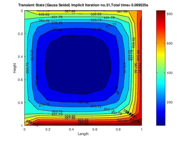
title_text=sprintf('Transient State (Gauss Seidel) Implicit Iteration no.%d,Total time= %fs',GS_iter,F);
title(title_text);
xlabel('Length');
ylabel('Height');
set(gca,'Ydir','reverse');
fprintf('Transient State Gauss Seidel Iteration no.%d\n',GS_iter);
OUTPUT:
7. TRANSIENT IMPLICIT SCHEME USING SUCCESSIVE OVER-RELAXATION METHOD:
CODE:
clear all;
close all;
clc;

%INPUTS
L=1;                  %Length of the Domain
q=1.4;
nx=10;                %number of grid points
ny=nx;

x=linspace(0,L,nx);
y=linspace(0,L,ny);
dx=x(2)-x(1);
dy=y(2)-y(1);
error=10000;
tol=1e-4;              %tolerance value
alpha=1.05;
dt=0.01;

%Given Temperatures at boundary
T_L=400;
T_T=600;
T_R=800;
T_B=900;
T=ones(nx,ny);
T(2:ny-1,1)= T_L;
T(2:ny-1,nx)= T_R;
T(1,2:nx-1)= T_T;
T(nx,2:ny-1)= T_B;

%Temperature at edges of the grid
T(1,1)= (T_T+T_L)/2;
T(nx,ny)= (T_R+T_B)/2;
T(1,ny)= (T_T+T_R)/2;
T(nx,1)= (T_L+T_B)/2;

k1=q*((dt)/(dx^2));
k2=q*((dt)/(dy^2));
[X,Y]= meshgrid(x,y);
Told=T;
Tprev=Told;

term1=(((2*k1)+(2*k2)+1)^(-1));
term2=k1*term1;
term3=k2*term1;

tic
SOR_iter=1;
for nt=1:1400
while(error>tol)
  for (i=2:nx-1)
    for (j=2:ny-1)
      A=(alpha*T(i-1,j))+((1-alpha)*Told(i-1,j))+Told(i+1,j);
      B=(alpha*T(i,j+1))+((1-alpha)*Told(i,j-1))+Told(i,j+1);
      T(i,j)=(Tprev(i,j)*term1)+(term2*A)+(term3*B);
    end
  end
  error=max(max(abs(Told-T)));
  Told=T;
  SOR_iter=SOR_iter+1;
end
Tprev=T;
endfor
F=toc;

figure(i)
[M,N]=contourf(x,y,T);
clabel(M,N);
colormap(jet);
colorbar;
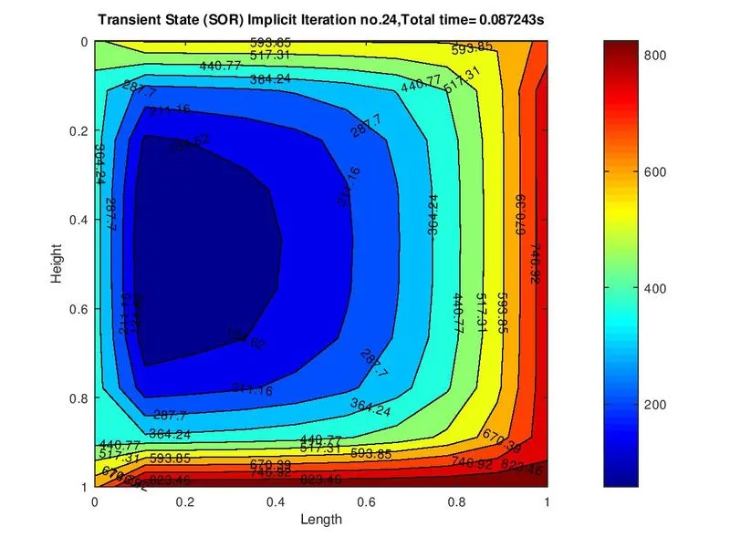
title_text=sprintf('Transient State (SOR) Implicit Iteration no.%d,Total time= %fs',SOR_iter,F);
title(title_text);
xlabel('Length');
ylabel('Height');
set(gca,'Ydir','reverse');
fprintf('Transient State SOR Iteration no.%d\n',SOR_iter);
OUTPUT:
Code Explanations:
- The temperatures ant boundary domain has been given. The temperatures at the edges of the domain has been calculated by taking average of the adjacent boundary temperatures.
- In Jacobi scheme, the initial T value is used in each iteration. In Gauss Seidel scheme, the value of previous time step 'Told' is used wherever possible. In Successive Over relaxation method, the Gauss Seidel equation is used with alpha as relaxation factor.
For SOR scheme: T(i,j)= (1-alpha)*Told(i,j)+ (alpha * Gauss Seidel scheme equation)
- Error is calculated as maximum value of difference between Told value and T value. After one iteration, Told value is reassigned the value of T within the while loop. The iteration is done till error value goes below the tolerance value.
- In Transient equations Tprev value is used. Tprev remains constant in a particulation time loop, whereas Told values are updated after each space loop.
Results:
For Steady State equation:
| Jacobi Method | Gauss Seidel Method | SOR Method | |
| Number of Iterations | 1884 | 1005 | 101 |
| Total time taken(seconds) | 41.26 | 21.48 | 2.66 |
For Transient equation(Explicit form):
| Transient Explicit Method | |
| Number of Iterations | 455 |
| Total time taken(seconds) | 1.33 |
For Transient equation(Implicit form):
| Jacobi Method | Gauss Seidel Method | SOR Method | |
| Number of Iterations | 53 | 31 | 24 |
| Total time taken(seconds) | 0.142 | 0.099 | 0.087 |
Hence from the aboce results,we conclude that Successive Over Relaxation method calculates the fasest, i.e. the eqaution converges quickly using SOR method, followed by Gauss Seidel Method, then Jacobi method for both Steady State and Transient Equation. Also, on comparing Implicit and Explicit method used in Transient Equation, we find Implicit method is faster than Explicit method with much less number of iterations required to converge the same equation.