Week 3 - Taylor table method and Matlab code

Objective:

To derive the 4th order approximations of the second-order derivative using Central difference, Skewed right-sided difference and Skewed left-sided difference.

Also, to write a program to evaluate the second-order derivative of the analytical function

`f(x)= e^x*cosx`

and to compare it with the 3 numerical approximations highlighted above.

Solution:

1. CENTRAL DIFFERENCE SCHEME:

Number of terms in Central Difference method=order of error+order of derivative-1

= 4+2-1= 5 terms

So, the numerical stencil under consideration will have 5 points, with information taken from both left and right side of i.

so, Fourth order approximation for second order derivative of the CDS is:

`(partial^2f)/(partialx^2)= a*f(i-2)+b*f(i-1)+c*f(i)+d*f(i+1)+e*f(i+2)` ....(1)

Expanding each term of the above equation using Taylor Series:

`f(i-2)= f(i)-(2trianglex)/(1!)*f'(i)+(2trianglex)^2/(2!)*f''(i)-(2trianglex)^3/(3!)f'''(i)+(2trianglex)^4/(4!)*f''''(i)+O(2trianglex)^5`

`b*f(i-1)= f(i)- (trianglex)/(1!)*f'(x)+(trianglex)^2/(2!)*f''(x)-(trianglex)^3/(3!)*f'''(x)+(trianglex)^4/(4!)*f''''(x)+O(trianglex)^5`

`c*f(i)=f(i)`

`d*f(i+1)= f(i)+ (trianglex)/(1!)*f'(x)+(trianglex)^2/(2!)*f''(x)+(trianglex)^3/(3!)*f'''(x)+(trianglex^4)/(4!)*f''''(x)+O(trianglex)^5`

`f(i+2)= f(i)+(2trianglex)/(1!)*f'(x)+(2trianglex)^2/(2!)*f''(x)+(2trianglex)^3/(3!)*f'''(x)+(2trianglex)^4/(4!)*f''''(x)+ O(2trianglex)^5``

Taking the above terms and putting them into Taylor Table:

	`f(i)`	`trianglex*f'(i)`	`trianglex^2*f''(i)`	`trianglex^3*f'''(i)`	`trianglex^4*f''''(i)`
a.f(i-2)	`a`	`-2a`	`(2^2a)/2`	`-(2^3a)/6`	`(2^4a)/24`
b.f(i-1)	`b`	`-b`	`(-1^3b)/6`	`(1^4b)/24`	`(1^2b)/24`
c.f(i)	`c`	`0`	`0`	`0`	`0`
d.f(i+1)	`d`	`d`	`(1^2d)/2`	`(-1^3d)/6`	`(1^4d)/24`
e.f(1+2)	`e`	`2e`	`(2^2e)/2`	`(2^3e)/6`	`(2^4e)/24`
SUM	0	0	1	0	0

As we have to find the 2nd order derivative, the sum of the coefficients of the second order terms will be equal to one, and the rest of the terms equates tio zero, as shown in the table.

We can solve the above system of equation using Matrix Inverse method:

A.X=B; X=`A^-1`.B; where: A is the coefficient matrix(5x5)

B is the matrix of the sums(1x5)

X is the matrix of the unknown terms[a;b;c;d;e](5x1)

on solving the equation we get the value of X as [0.0833;1.3333;-2.5000;1.3333;-0.0833]

So, a=0.0833 ; c=1.3333 ; d=-2.5000 ; e=1.3333 ; g=-0.8333

Now, substituting these values in eqt (1) we get:

`(d^2f(x))/dx^2= -0.0833*f(i-2)+ 1.333*f(i-1)- 2.5000*f(i)+ 1.3333*f(i+1)- 0.0833*f(i+2)`

2. SKEWED RGHT DIFFERENCE SCHEME:

Number of terms for this method will be simply equal to: order of error+ order of derivative

=4+2 = 6

Thus, there will be 6 terms in the approximation equation of Skewed Right side scheme, with all the points situated to the right side of 'i' (the point where we need to calculate the second order derivative)in the numerical stencil. Hence, the equation will; look like following:

`(partial^2x)/(partialx^2)= a*f(i)+ b*f(i+1)+ c*f(i+2)+ d*f(i+3)+ e*f(i+4)+ g*f(i+5)` ......(2)

Taylor series expansion will be applied to expand each term. The Taylor table would look like following:

	`f(i)`	`trianglex*f'(i)`	`trianglex^2*f''(i)`	`trianglex^3.f'''(i)`	`trianglex^4*f''''(i)`	`trianglex^5f'''''(i)`
`a*f(i)`	`a`	`0`	`0`	`0`	`0`	`0`
`b*f(i+1)`	`b`	`b`	`(1^2b)/2`	`(1^3b)/6`	`(1^4b)/24`	`(1^5b)/120`
`c*f(i+2)`	`c`	`2c`	`(2^2c)/2`	`(2^3c)/6`	`(2^4c)/24`	`(2^5c)/120`
`d*f(i+3)`	`d`	`3d`	`(3^2d)/2`	`(3^3d)/6`	`(3^4d)/24`	`(3^5d)/120`
`e*f(i+4)`	`e`	`4e`	`(4^2e)/2`	`(4^3e)/6`	`(4^4e)/24`	`(4^5e)/120`
`g*f(i+5)`	`g`	`5g`	`(5^2g)/2`	`(5^3g)/6`	`(5^4g)/24`	`(5^5g)/120`
SUM	0	0	0	1	0	0

Now, as used in the previous method, we again use Inverse Matrixmultiplication method to find the values of the unknowns, which comes out to be [3.7500;-12.8333;17.8333;-13.0000;5.0833;-0.8333].

So, a=3.7500; b=-12.8333 ;c=17.8333 ;d=-13.0000 ;e=5.0833 ;g=-0.8333

Now, substituting these values in eqt (2) we get:

`(d^2f(x))/dx^2= 3.7500*f(i)- 12.8333*f(i+1)+ 17.8333*f(i+2)- 13.0000*f(i+3)+ 5.0833*f(i+4)- 0.8333*f(i+5)`

3. SKEWED LEFT SIDE DIFFERENCE SCHEME:

Number of terms for this method will be again equal to: order of error+ order of derivative

=4+2 = 6

Same procedure will be followed as done in the right sided skewed scheme, only difference being that the nodes are now situated to the left side of 'i' in the numerical stencil. The fourth order approximation equation usinf Left skewed scheme will look like:

`(partial^2x)/(partialx^2)= a*f(i)+ b*f(i-1)+ c*f(i-2)+ d*f(i-3)+ e*f(i-4)+ g*f(i-5)` ......(3)

Hence, the node width or 'dx' will be `'-trianglex'`, making the odd derivative terms '-ve' and the even derivative terms '+ve'.

Hence, the Taylor table will look like following:

	`f(i)`	`trianglex*f'(i)`	`trianglex^2*f''(i)`	`trianglex^3.f'''(i)`	`trianglex^4*f''''(i)`	`trianglex^5f'''''(i)`
`a*f(i)`	`a`	`0`	`0`	`0`	`0`	`0`
`b*f(i-1)`	`b`	`-b`	`(1^2b)/2`	`-(1^3b)/6`	`(1^4b)/24`	`-(1^5b)/120`
`c*f(i-2)`	`c`	`-2c`	`(2^2c)/2`	`-(2^3c)/6`	`(2^4c)/24`	`-(2^5c)/120`
`d*f(i-3)`	`d`	`-3d`	`(3^2d)/2`	`-(3^3d)/6`	`(3^4d)/24`	`-(3^5d)/120`
`e*f(i-4)`	`e`	`-4e`	`(4^2e)/2`	`-(4^3e)/6`	`(4^4e)/24`	`-(4^5e)/120`
`g*f(i-5)`	`g`	`-5g`	`(5^2g)/2`	`-(5^3g)/6`	`(5^4g)/24`	`-(5^5g)/120`
SUM	0	0	0	1	0	0

Using the same method to find the unknowns, we get the following result:

a=3.7500; b=-12.8333 ;c=17.8333 ;d=-13.0000 ;e=5.0833 ;g=-0.8333

Now, substituting these values in eqt (3) we get:

`(d^2f(x))/dx^2= 3.7500*f(i)- 12.8333*f(i-1)+ 17.8333*f(i-2)- 13.0000*f(i-3)+ 5.0833*f(i-4)- 0.8333*f(i-5)`

MATLAB CODE:

clear all;
close all;
clc;

% Analytical function f(x)= exp(x)*cos(x)
%f'(x)= 2*exp(x)*(-sin(x))

x=pi/3;
dx= linspace(pi/4,pi/400,20);

%Fourth Order Approximation
for i=1:length(dx)
  central_diff(i)=((-0.0833)*(exp(x-(2*dx(i))))*(cos(x-(2*dx(i)))))+((1.3333)*(exp(x-dx(i)))*((cos(x-dx(i))))+(-2.5)*(exp(x))*(cos(x)))+((1.3333)*(exp(x+dx(i)))*(cos(x+dx(i))))+((-0.0833)*(exp(x+(2*dx(i))))*(cos(x+(2*dx(i)))))/((dx(i))^2);
  skewed_right(i)=((3.75)*(exp(x))*(cos(x)))+((-12.8333)*(exp(x+dx(i)))*(cos(x+dx(i))))+((17.8333)*(exp(x+(2*dx(i))))*(cos(x+(2*dx(i)))))+((-13)*(exp(x+(3*dx(i))))*(cos(x+(3*dx(i)))))+((5.0833)*(exp(x+(4*dx(i))))*(cos(x+(4*dx(i)))))+((-0.8333)*(exp(x+(5*dx(i))))*(cos(x+(5*dx(i)))))/((dx(i))^2);
  skewed_left(i)=((3.75)*(exp(x))*(cos(x)))+((-12.8333)*(exp(x-dx(i)))*(cos(x-dx(i))))+((17.8333)*(exp(x-(2*dx(i))))*(cos(x-(2*dx(i)))))+((-13)*(exp(x-(3*dx(i))))*(cos(x-(3*dx(i)))))+((5.0833)*(exp(x-(4*dx(i))))*(cos(x-(4*dx(i)))))+((-0.8333)*(exp(x-(5*dx(i))))*(cos(x-(5*dx(i)))))/((dx(i))^2);
  
end  

Derivative= -2*exp(x)*sin(x);
error_cds= abs(central_diff-Derivative);
error_srsd= abs(skewed_right-Derivative);
error_slsd= abs(skewed_left-Derivative);



figure(1)
loglog(dx,error_cds,'linewidth',3);
grid on;
hold on;
loglog(dx,error_srsd,'linewidth',3);
hold on;
loglog(dx,error_slsd,'linewidth',3);
xlabel('dx');
ylabel('Error due to dx');
title('Plot for Fourth Order Approximation for Second Order Derivative under different schemes');
legend('Central Differencing Scheme','Skewed Right Side Differencing Scheme','Skewed Left Side DIfferencing Scheme')

Terms used in the above code:

*central_diff(i)- to calculate the central difference approximation using the approximation equation

*skewed_right(i)- to calculate the Skewed Right side difference approximation

*skewed_left(i)- to calculate the Skewed left side difference approximation

'error_cds', 'error_srsd' and 'error_slsd' are the error terms(Analytical Derivative-Numerically calculated derivative) for Central Difference, Skewed Right Side and Skewed Left Side methods respectively.

CONCLUSION:

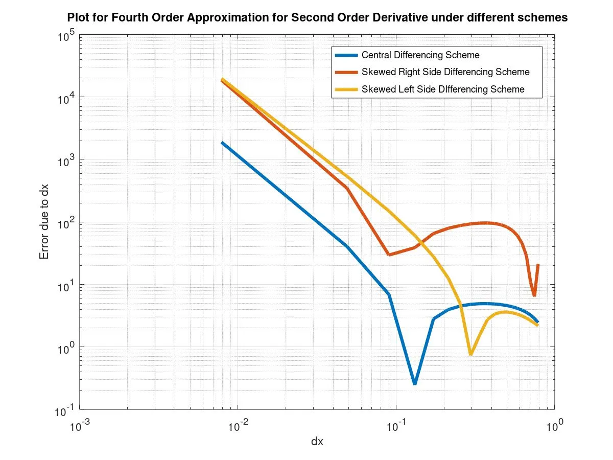
The result of the MATLAB program is shown in the above plot. The plot shows the 'error' vs ' the grid size' for Central Difference, Skewed Right side and Skewed Left side method. The plot shows that lowering the value of deltax decreases the error, but lowering it below a certain point results in increasing error value.

From the plot, it is also clear that the 'Central Difference method' has lower average error value as compared to the other two schemes. The next, most accurate scheme here is the Left skewed scheme, followed by the right skewed scheme. This makes sense, as Central Difference scheme takes reference points from both side of the point where derivative is to be calculated, as opposed to right amd left skewed schemes, which only considers points on the right side or left side respectively.

Even though Central Difference Scheme is the most accurate scheme, it is not practically possible to use it in every condition. As this scheme requires nodal points at both sides of 'i', at some situations, like at the boundary of a grid, Central Difference Scheme qill not yeild results. Hence, the scheme to be used to entirely problem dependant.