Week 5.1 - Mid term project - Solving the steady and unsteady 2D heat conduction problem

WEEK 5.1-CHALLENGE -DETAILED REPORT

OBJECTIVES:

1. Steady state analysis & Transient State Analysis

Solve the 2D heat conduction equation by using the point iterative techniques that were taught in the class. The Boundary conditions for the problem are as follows;

Top Boundary = 600 K

Bottom Boundary = 900 K

Left Boundary = 400 K

Right Boundary = 800 K

You will implement the following methods for solving implicit equations.

• Jacobi
• Gauss-seidel
• Successive over-relaxation

absolute error criteria is 1e-4

First I wrote programe for steady state

MATLAB Programe:

(a) Jacobi Method

% steady state
clear all
close all
clc

% inputs
nx=11 % no of nodes in x direction
ny=nx  % no of nodes in y direction
% giving temperature profile
T=300*ones(nx,ny)
% meshing
x=linspace(0,1,nx) % meshing in x direction
dx=x(2)-x(1)       % distance between two adjacent nodes in x direction
y=linspace(0,1,ny)  % meshing in y direction
dy=y(2)-y(1)        % distance between two adjacent nodes in y direction
% applying boundary condition
T(:,1)=400 % left boundary condition
T(:,end)=800 % right boundary condition
T(1,:)= 600 % top boundary layer
T(end,:)=900 % bottom boundary layer
T(1,1)=(T(1,2)+T(2,1))/2
T(end,1)=(T(end-1,1)+T(end,2))/2
T(end,end)=(T(end,end-1)+T(end-1,end))/2
T(1,end)=(T(1,end-1)+T(2,end))/2


% applying initial conditions

Told=T
T_initial=Told
% giving error and tolerence
iterative_solver=3
error=1e9
tol=1e-4
k=(dx^2*dy^2)/(2*(dx^2+dy^2))

% jacobi method

if iterative_solver==1
    jacobi_iter=1
    % convergence loop
    while (error>tol)
        
        %space loop
         for i=2:nx-1 % opening for loop for x axis
             for j=2:ny-1 % opening for loop for y axis
                 
                 T(i,j)=k*(Told(i-1,j)+Told(i+1,j))/dx^2 +k*(Told(i,j-1)+Told(i,j+1))/dy^2
             end % ending 2nd for loop
         end     % ending 1st for loop
         error=max(max(abs(Told-T)))  %calculating error
         Told=T  %updating Told
         jacobi_iter=jacobi_iter+1 %giving increment of iteration number
         
         % plotting
         figure(1);
         %contourplot(x,T)
         [c,h]=contourf(T)
         clabel(c,h)
         colorbar('southoutside')
         set(gca,'ydir','reverse')
         xlabel('X axis')
         ylabel('Y axis')
         title_text=sprintf('iteration number=%d',jacobi_iter)
    title( title_text)
    end
end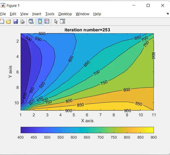

Contour of temperature with Jacobi method for steady state

(b) Gauss-Siedel Method

% Gauss-Siedel method

if iterative_solver==2
    gs_iter=0;
    % convergence loop
    while (error>tol)
        
        %space loop
         for i=2:nx-1 % opening for loop for x axis
             for j=2:ny-1 % opening for loop for y axis
                 
                 T(i,j)=k*(T(i-1,j)+Told(i+1,j))/dx^2 +k*(T(i,j-1)+Told(i,j+1))/dy^2
             end % ending 2nd for loop
         end     % ending 1st for loop
         error=max(max(abs(Told-T)))  %calculating error
         Told=T  %updating Told
         gs_iter=gs_iter+1 %giving increment of iteration number
         
         % plotting
         figure(1);
         %contourplot(x,T)
         [c,h]=contourf(T)
         clabel(c,h)
         colorbar('southoutside')
         set(gca,'ydir','reverse')
         xlabel('X axis')
         ylabel('Y axis')
         title_text=sprintf('iteration number=%d',gs_iter)
    title( title_text)
    end
end
     

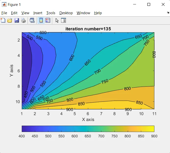
Contour of temperature with Gauss-Siedel method for steady state

(c) SOR Method

% SOR method
w=1.5
if iterative_solver==3
    sor_iter=0;
    % convergence loop
    while (error>tol)
        
        %space loop
         for i=2:nx-1 % opening for loop for x axis
             for j=2:ny-1 % opening for loop for y axis
                 
                 Tgs(i,j)=k*(T(i-1,j)+Told(i+1,j))/dx^2 +k*(T(i,j-1)+Told(i,j+1))/dy^2
                 T(i,j)=(1-w)*Told(i,j)+w*Tgs(i,j)
             end % ending 2nd for loop
         end     % ending 1st for loop
         error=max(max(abs(Told-T)))  %calculating error
         Told=T  %updating Told
         sor_iter=sor_iter+1 %giving increment of iteration number
         
         % plotting
         figure(1);
         %contourplot(x,T)
         [c,h]=contourf(T)% giving contour
         clabel(c,h)
         colorbar('southoutside')% giving colorbat at bottom
         set(gca,'ydir','reverse')% reversing y axis
         xlabel('X axis') % labeling of x axis
         ylabel('Y axis')  % labeling of y axis
         title_text=sprintf('iteration number=%d',sor_iter) %giving title for plot
    title( title_text)
    end %  ending while loop 
end     % ending if loop

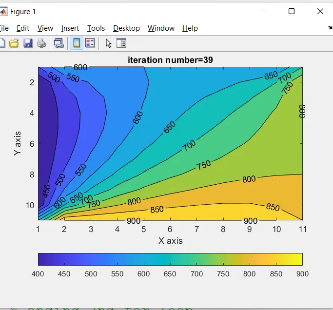
Contour of temperature with SOR method for steady state

ITERATIVE METHOD	NUMBER OF ITERATIONS
Jacobi	253
Gauss-Siedel	135
SOR	39

(b) Transient-explicit

Programme:

% transient case-Explicit
clear all %clearing workspcae
close all %closing figures and plots
clc  %clearing screen

% inputs
nx=11 % no of nodes in x direction
ny=nx  % no of nodes in y direction
% giving temperature profile
T=300*ones(nx,ny);
% meshing
x=linspace(0,1,nx); % meshing in x direction
dx=x(2)-x(1) ;      % distance between two adjacent nodes in x direction
y=linspace(0,1,ny);  % meshing in y direction
dy=y(2)-y(1);        % distance between two adjacent nodes in y direction
% applying boundary condition
T(:,1)=400; % left boundary condition
T(:,end)=800; % right boundary condition
T(1,:)= 600; % top boundary layer
T(end,:)=900; % bottom boundary layer
T(1,1)=(T(1,2)+T(2,1))/2; %temperature at the 1st node
T(end,1)=(T(end-1,1)+T(end,2))/2;
T(end,end)=(T(end,end-1)+T(end-1,end))/2;
T(1,end)=(T(1,end-1)+T(2,end))/2;

% applying initial conditions

T_old=T;
T_initial=T_old;
alpha=1.5;
dt=0.001; %duration of timestep
nt=500;% total no of timestep
k1=(alpha* dt)/(dx^2); % define k1
k2=(alpha* dt)/(dy^2);  % define k2
    %time loop
    for m=1:nt
        
        %space loop
         for i=2:nx-1 % opening for loop for x axis
             for j=2:ny-1 % opening for loop for y axis
                 term1=T_old(i,j);
               term2=k1*(T_old(i-1,j)+T_old(i+1,j)-2*(term1));
               term3=k2*(T_old(i,j+1)+T_old(i,j-1)-2*(term1));
               T(i,j)=term1+term2+term3; % equation of temperature
           end  
       end
      
         error=max(max(abs(T_old-T))) ; %calculating error
         T_old=T ; %updating Told

         % plotting
         figure(1)
         %contourplot(x,T)
         [c,h]=contourf(T);
         clabel(c,h);
         colorbar('southoutside');
         set(gca,'ydir','reverse');
         xlabel('X axis');% giving naming to x axis
         ylabel('Y axis');% giving naming to y axis
         title_text=sprintf('explicit method,running time=%0.4f',dt*m);% giving title to plot
         title(title_text);
    end % ending for loop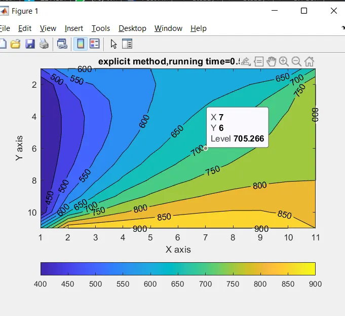

Plot for transient explicit case

Transient-Implicit case

PROGRAMME:

% Transient state-implicit
clear all % clearing workspace
close all % closing figures and plots
clc      % clearing screen

% inputs
nx=10; % no of nodes in x direction
ny=10 ; % no of nodes in y direction
% giving temperature profile
T=300*ones(nx,ny);
% meshing
x=linspace(0,1,nx); % meshing in x direction
dx=x(2)-x(1) ;      % distance between two adjacent nodes in x direction
y=linspace(0,1,ny);  % meshing in y direction
dy=y(2)-y(1);        % distance between two adjacent nodes in y direction
% applying boundary condition
T(:,1)=400; % left boundary condition
T(:,end)=800; % right boundary condition
T(1,:)= 600; % top boundary layer
T(end,:)=900 ;% bottom boundary layer
T(1,1)=(T(1,2)+T(2,1))/2;
T(end,1)=(T(end-1,1)+T(end,2))/2;
T(end,end)=(T(end,end-1)+T(end-1,end))/2;
T(1,end)=(T(1,end-1)+T(2,end))/2;


% applying initial conditions

T_old=T;
T_initial=T_old;
T_prev=T;
% giving error and tolerence
%iterative_solver=3;
%error=1e9;
tol=1e-9;
nt=1400;
dt=0.01;
alpha=1.4;
k1=alpha*(dt/(dx^2)); % define k1
k2=alpha*(dt/(dy^2));  % define k2
CFL = k1 + k2;

iterative_solver=input('iterative method=');
% jacobi method

if (iterative_solver==1)
    jacobi_iter=1;
    % time loop
    for m=1:nt
        error=1e9;% giving error    
    % convergence loop
    while(error>tol)
        %space loop
         for i=2:nx-1 % opening for loop for x axis
             for j=2:ny-1 % opening for loop for y axis
                 term1=(1+(2*k1)+(2*k2))^-1;
                 term2=k1*term1;
                 term3=k2*term1;
                 
                 h=T_old(i-1,j)+T_old(i+1,j);
                 g=T_old(i,j-1)+T_old(i,j+1);
                 
                 T(i,j)=(T_prev(i,j)*term1)+(term2*h)+(term3*g);
                 %T(i,j)=term1*T_prev(i,j)+term2*(T_old(i-1,j)+T_old(i+1,j))+term3*(T_old(i,j+1)+T_old(i,j-1));
             end % ending 2nd for loop
          end     % ending 1st for loop
         error=max(max(abs(T_old-T)));  %calculating error
         T_old=T;  %updating Told
         jacobi_iter=jacobi_iter+1; %giving increment of iteration number
    end
        T_prev=T;
    end
    % plotting
         figure(1)
         %contourplot(x,T)
         [c,h]=contourf(T);
         clabel(c,h);
         colorbar('southoutside');
         set(gca,'ydir','reverse');
         xlabel('X axis');
         ylabel('Y axis');
         title_text=sprintf('iteration number=%d',jacobi_iter);
    title( title_text);
    
end
        
 



% Gauss-Siedel method

if iterative_solver==2
    gs_iter=1;
    % time loop
    for m=1:nt
        error=1e9; 
    
    % convergence loop
    while (error>tol)
        
        %space loop
         for i=2:nx-1 % opening for loop for x axis
             for j=2:ny-1 % opening for loop for y axis
                 term1=(1+(2*k1)+(2*k2))^-1;
                 term2=k1*term1;
                 term3=k2*term1;
                 
                 h=T(i-1,j)+T_old(i+1,j);
                 g=T(i,j-1)+T_old(i,j+1);
                 
                 T(i,j)=(T_prev(i,j)*term1)+(term2*h)+(term3*g);
                 %T(i,j)=k*(T(i-1,j)+T_old(i+1,j))/dx^2 +k*(T(i,j-1)+T_old(i,j+1))/dy^2
             end % ending 2nd for loop
         end     % ending 1st for loop
         error=max(max(abs(T_old-T)));  %calculating error
         T_old=T;  %updating Told
         gs_iter=gs_iter+1; %giving increment of iteration number
    end
    T_prev=T;
    end
         % plotting
         figure(1);
         %contourplot(x,T)
         [c,h]=contourf(T);
         clabel(c,h);
         colorbar('southoutside');
         set(gca,'ydir','reverse');
         xlabel('X axis');
         ylabel('Y axis');
         title_text=sprintf('iteration number=%d',gs_iter);
    title( title_text);
    
end
     


% SOR method
omega=1.2;
if iterative_solver==3
    sor_iter=1;
    % time loop
    for m=1:nt
        error=1e9; 
    % convergence loop
    while (error>tol)
        
        %space loop
         for i=2:nx-1 % opening for loop for x axis
             for j=2:ny-1 % opening for loop for y axis
                 term1=(1+(2*k1)+(2*k2))^-1;
                 term2=k1*term1;
                 term3=k2*term1;
                 
                 h=T(i-1,j)+T_old(i+1,j);
                 g=T(i,j-1)+T_old(i,j+1);
                 
                 Tgs=(T_prev(i,j)*term1)+(term2*h)+(term3*g);
                 T(i,j)=((1-omega)*T_old(i,j))+(omega*Tgs);
             end % ending 2nd for loop
         end     % ending 1st for loop
         error=max(max(abs(T_old-T)));  %calculating error
         T_old=T;  %updating Told
         sor_iter=sor_iter+1; %giving increment of iteration number
    end
    T_prev=T;
    end
         % plotting
         figure(1);
         %contourplot(x,T)
         [c,h]=contourf(T);% giving contour
         clabel(c,h);
         colorbar('southoutside');% giving colorbat at bottom
         set(gca,'ydir','reverse');% reversing y axis
         xlabel('X axis'); % labeling of x axis
         ylabel('Y axis');  % labeling of y axis
         title_text=sprintf('iteration number=%d',sor_iter); %giving title for plot
    title( title_text);
end %  ending while loop 
     

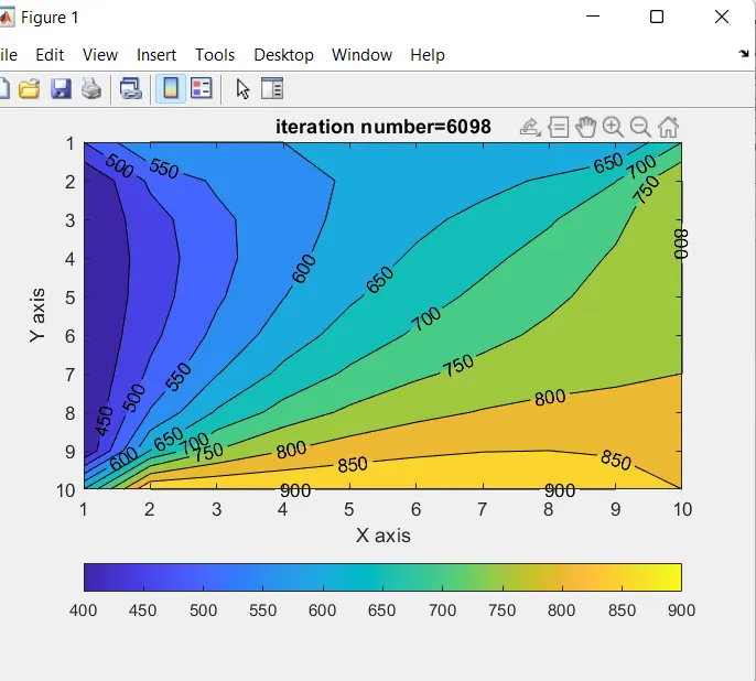
plot for implicit -Jacobi method

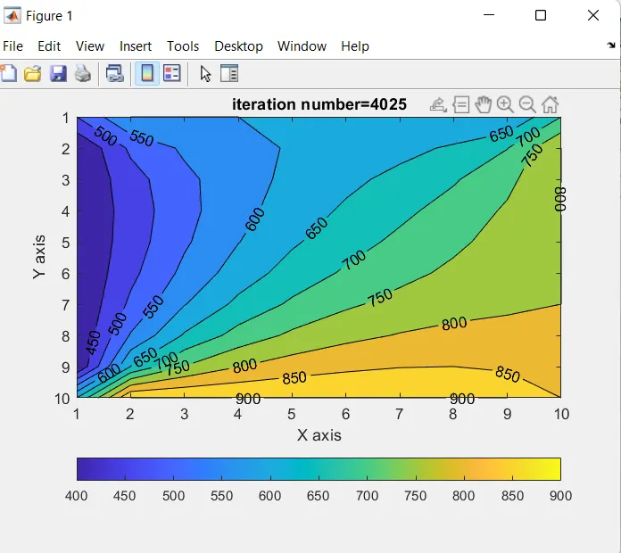
plot for implicit -Gauss-Siedel method

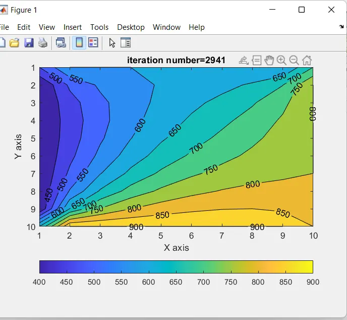
plot for implicit -SOR method

Method	Number of Iterations
Jacobi	6098
Gauss-Siedel	4025
SOR	2941

CONCLUSIONS:

*Steady state and transient case simulation done

*Both implicit case and explicit case analysis done for transient case

*Comaperd the no of iterations in Jacobi, Gauss-Siedel and SOR Methods.

*SOR Method takes very less no of iterations while Jacobi method takes large no of iterations