Week 5.1 - Mid term project - Solving the steady and unsteady 2D heat conduction problem
Objectives of the assignment
- To write a code in MATLAB to solve for the 2D heat conduction equation in Steady-state for the given boundary conditions using the point iterative techniques.
- To write a code in MATLAB to solve for the 2D heat conduction equation in Transient state in the explicit method.
- To write a code in MATLAB to solve for the 2D heat conduction equation in Transient state in the implicit method using the point iterative techniques.
The problem statement and assumptions:
- For the given problem statement, the Specimen area is a square.
- We assume that nx = ny [No. of points on x-direction is equal to no. of points in y-direction]
- We assume nx = ny = 10
- Given Boundary Conditions are
Left = 400k
Right = 600k
Top = 800k
Bottom = 900k - Let’s assume that apart from the boundary conditions, all other nodes are given an initial temperature of 300k.
- We predefine an error term and a guess the temperature values and then use iterative solvers to arrive at a value for the temperature at each node.
2D Steady-state heat conduction equation:
The equation is as follows:
`(del^2T)/(delx^2) + (del^2T)/(dely^2) = 0`
By discretizing the above equation using Central Difference Method, we've:
`Tp = (1/k) [((Tl+Tr)/ (Delta x^2)) + ((Tt+Tb)/(Delta y^2))]`
where `k = 2((Delta x^2 + Delta y^2)/ (Delta x^2 Delta y^2))`
The following code is the MATLAB code to solve for the 2D steady-state heat conduction in the implicit method using Jacobi,Gauss Seidal and Successive Over-Relaxation iterative solvers.
close all
clear all
clc

%Solving the Steady state 2D heat conduction (Jacobi Method)

%Input Parameters
%Number of grid points
nx = 10;
ny = nx;

x = linspace(0,1,nx);
y = linspace(0,1,ny);

dx = x(2) - x(1);
dy = y(2) - y(1);

%Absolute error criteria > tolerance
error = 9e9;
tolerance = 1e-4;

%Defining Boundary conditions
T_L = 400;
T_T = 600;
T_R = 800;
T_B = 900;

%Initial Temperature (and Assumed first set of guess Temperature values)
T = (300*ones(nx,ny));

T(2:ny - 1, 1)  = T_L;
T(2:ny - 1, nx) = T_R;
T(1, 2:nx - 1)  = T_T;
T(ny, 2:nx - 1) = T_B;

%Calculating Average temperature at corners
T(1,ny) = (T_T + T_L)/2;
T(nx,1) = (T_R + T_B)/2;
T(nx,ny) = (T_T + T_R)/2;
T(1,1) = (T_L + T_B)/2;

%defining the K term..
K =  (dx^2*dy^2)/(2*(dx^2+dy^2));

%Assigning orginal values to T
T_initial = T;
T_old = T;

%Calculation of 2D steady heat conduction EQUATION by JACOBI method

jacobi_iteration = 1;

    while(error > tolerance)

        for i = 2:nx - 1

            for j = 2:ny - 1

            %calculating the temperature of a point using Jacobi method
            Term1 = (T_old(i-1,j)+T_old(i+1,j))/(dx^2);

            Term2 = (T_old(i,j-1)+T_old(i,j+1))/(dy^2);

            T(i,j) = K*(Term1 + Term2);

            end

        end

        error = max(max(abs(T_old - T)));
        T_old = T;
        jacobi_iteration = jacobi_iteration + 1;

    end

%Plotting
figure(1)
contourf(x,y,T)
clabel(contourf(x,y,T))
colorbar
colormap(jet)
set(gca, 'ydir', 'reverse')

xlabel('X-Axis')
ylabel('Y-Axis')
title(sprintf('No. of Jacobi Iterations(IMPLICIT) = %d', jacobi_iteration));
pause(0.03);

%Reinitialising the temperature, error and iterations count and repeat the above steps for Gauss-Seidel method.
T = T_initial;
T_old = T;

%Absolute error criteria > tolerance
error = 9e9;

GS_iteration = 1;

    while(error > tolerance)

        for i = 2:nx - 1

            for j = 2:ny - 1

            %calculating the temperature of a point using Gauss Seidal method
            Term1 = (T(i-1,j)+T_old(i+1,j))/(dx^2);

            Term2 = (T(i,j-1)+T_old(i,j+1))/(dy^2);

            T(i,j) = K*(Term1 + Term2);

            end

        end

        error = max(max(abs(T_old - T)));
        T_old = T;
        GS_iteration = GS_iteration + 1;

    end

%Plotting
figure(2)
contourf(x,y,T)
clabel(contourf(x,y,T))
colorbar
colormap(jet)
set(gca, 'ydir', 'reverse')

xlabel('X-Axis')
ylabel('Y-Axis')
title(sprintf('No. of GaussSeidal Iterations(IMPLICIT) = %d', GS_iteration));
pause(0.03);

%Reinitialising the temperature, error and iterations count and repeat the above steps for SOR method.
T = T_initial;
T_old = T;

%Absolute error criteria > tolerance
error = 9e9;

SOR_iteration = 1;

%Relaxation Factor (Over Relaxed Condition)
Alpha = 1.2;

    while(error > tolerance)

        for i = 2:nx - 1

            for j = 2:ny - 1

            %calculating the temperature of a point using SOR method
            Term1 = (T(i-1,j)+T_old(i+1,j))/(dx^2);

            Term2 = (T(i,j-1)+T_old(i,j+1))/(dy^2);

            T(i,j) = K*(Term1 + Term2);

            T(i,j) = T_old(i,j)*(1-Alpha)+(Alpha*T(i,j));

            end

        end

        error = max(max(abs(T_old - T)));
        T_old = T;
        SOR_iteration = SOR_iteration + 1;

    end

%Plotting
figure(3)
contourf(x,y,T)
clabel(contourf(x,y,T))
colorbar
colormap(jet)
set(gca, 'ydir', 'reverse')

xlabel('X-Axis')
ylabel('Y-Axis')
title(sprintf('No. of SOR Iterations(IMPLICIT) = %d', SOR_iteration));
pause(0.03);
Resuts:
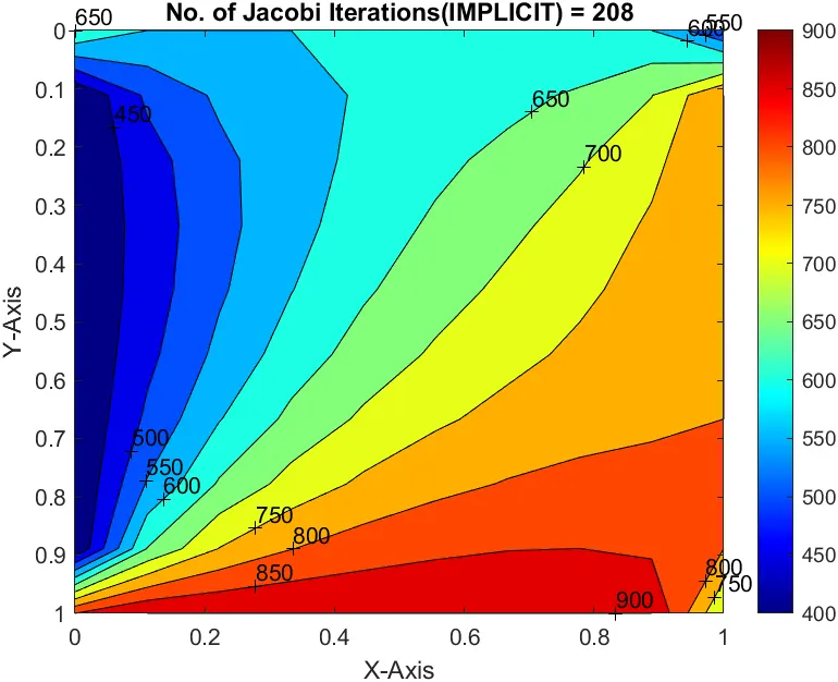
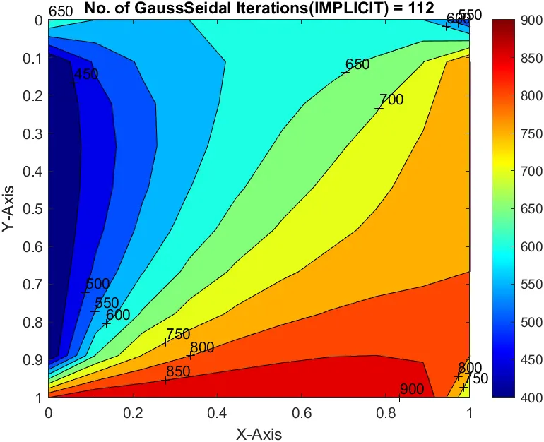
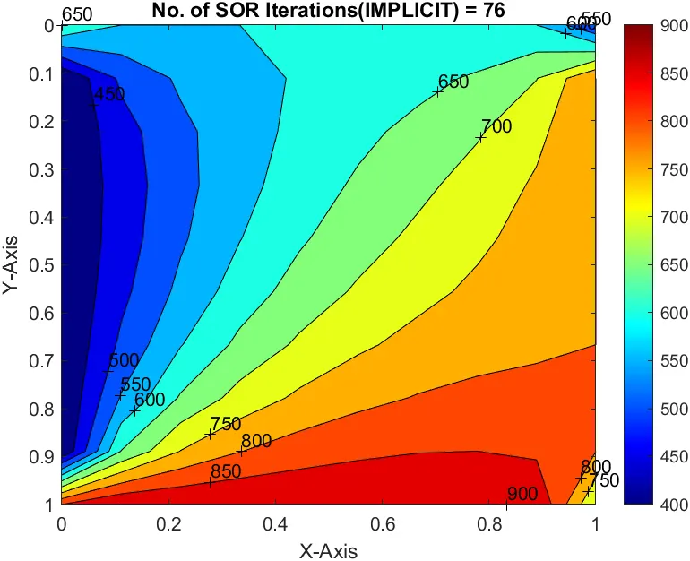
2D Transient state heat conduction:
The 2D heat conduction equation in the transient state is as follows:
`(∂T)/(∂t) = α((del^2T)/(delx^2))+((del^2T)/(dely^2))`
Where, `alpha` is the thermal diffusivity.
if we discretize the above equation using Central Difference Method Implicitly, we get
`(T_P^(n+1))=(T_P^n)-αdeltat[((T_(R)-2T_(P)+T_(L))/(deltax^2))+((T_(T)-2T_(P)+T_(B))/(deltay^2))]^(n+1)`
if we simply further we get
`(T_P^(n+1))=(1/(1+k1+k2)) (T_P^n + k1(T_(R)+T_(L))^(n+1) + k2(T_(T)+T_(B))^(n+1))`
where,
`k1 = alpha((deltat)/(deltax^2)) and k2 = alpha((deltat)/(deltay^2))`
The following code is the MATLAB code to solve for the 2D Transient/Unsteady-state heat conduction in the implicit method using Jacobi,Gauss Seidal and Successive Over-Relaxation iterative solvers.
%Solving the Transient state 2D heat conduction through Implicit method (Jacobi,GS&SOR Method)

close all
clear all
clc

%Input Parameters
%Number of grid points
nx = 10;
ny = nx;

x = linspace(0,1,nx);
y = linspace(0,1,ny);

dx = x(2) - x(1);
dy = y(2) - y(1);

%defining the time marching steps.
t = 1000;
dt = 10;

%Defining Boundary conditions
T_L = 400;
T_T = 600;
T_R = 800;
T_B = 900;

%Initial Temperature (and Assumed first set of guess Temperature values)
T = 300*ones(nx,ny);

T(2:ny - 1,1)  = T_L;
T(2:ny - 1, nx) = T_R;
T(1, 2:nx - 1)  = T_T;
T(ny, 2:nx - 1) = T_B;

%Calculating Average temperature at corners
T(1,ny) = (T_T + T_L)/2;
T(nx,1) = (T_R + T_B)/2;
T(nx,ny) = (T_T + T_R)/2;
T(1,1) = (T_L + T_B)/2;

%Assigning orginal values to T
T_initial = T;
T_old = T;

%defining the thermal diffusivity (Ability of a material to conduct the heat transfer)
alpha = 1.2;

%initialising the k1 and k2 for future simplifications
k1 = alpha*(dt/(dx^2));
k2 = alpha*(dt/(dy^2));

%Absolute error criteria > tolerance
error = 1;
tolerance = 1e-4;

%Calculation of 2D Transient state heat conduction EQUATION by JACOBI method

jacobi_iteration = 1;

%Initiating the time loop.
for nt = 1:1400

    while error > tolerance

        %Initiating the Space loop.
        for i = 2:nx - 1

            for j = 2:ny - 1

            %calculating the temperature of a point using Jacobi method
            Term1 = 1/(1+(2*k1)+(2*k2));

            Term2 = k1*Term1;

            Term3 = k2*Term1;

            H = (T_old((i-1),j)+T_old((i+1),j));

            V = (T_old(i,(j-1))+T_old(i,(j+1)));

            T(i,j) =(T_initial(i,j)*Term1)+(H*Term2)+(V*Term3);

            end

        end

        error = max(max(abs(T_old - T)));
        T_old = T;
        jacobi_iteration = jacobi_iteration + 1;

    end

%updating the t_initial.
T_initial = T;

end

%Plotting
figure(1)
[c,h] = contourf(x,y,T);
clabel(c,h);
colorbar
colormap(jet)
set(gca, 'ydir', 'reverse')

xlabel('X-Axis')
ylabel('Y-Axis')
title({['2D  Heat Conduction in Transient State - Implicit method using Jacobi method.'],['Number of iterations = ',num2str(jacobi_iteration)]});


%Calculation of 2D Transient state heat conduction EQUATION by GS method
%Reinitiating error value and
error = 1

GS_iteration = 1;

%Initiating the time loop.
for nt = 1:1400

    while error > tolerance

        %Initiating the Space loop.
        for i = 2:nx - 1

            for j = 2:ny - 1

            %calculating the temperature of a point using Jacobi method
            Term1 = 1/(1+(2*k1)+(2*k2));

            Term2 = k1*Term1;

            Term3 = k2*Term1;

            H = (T((i-1),j)+T_old((i+1),j));

            V = (T(i,(j-1))+T_old(i,(j+1)));

            T(i,j) =(T_initial(i,j)*Term1)+(H*Term2)+(V*Term3);

            end

        end

        error = max(max(abs(T_old - T)));
        T_old = T;
        GS_iteration = GS_iteration + 1;

    end

%updating the t_initial.
T_initial = T;

end

%Plotting
figure(2)
[c,h] = contourf(x,y,T);
clabel(c,h);
colorbar
colormap(jet)
set(gca, 'ydir', 'reverse')

xlabel('X-Axis')
ylabel('Y-Axis')
title({['2D  Heat Conduction in Transient State - Implicit method using GS method.'],['Number of iterations = ',num2str(GS_iteration)]});

%Calculation of 2D Transient state heat conduction EQUATION by SOR method
%Reinitiating error value and
error = 1

SOR_iteration = 1;

%defining the Omega value i.e., thermal diffusivity (Ability of a
%material to conduct the heat transfer)
omega = 1.2

%Initiating the time loop.
for nt = 1:1400

    while error > tolerance

        %Initiating the Space loop.
        for i = 2:nx - 1

            for j = 2:ny - 1

            %calculating the temperature of a point using Jacobi method
            Term1 = 1/(1+(2*k1)+(2*k2));

            Term2 = k1*Term1;

            Term3 = k2*Term1;

            H = (T((i-1),j)+T_old((i+1),j));

            V = (T(i,(j-1))+T_old(i,(j+1)));

            T(i,j) =(T_initial(i,j)*Term1)+(H*Term2)+(V*Term3);

            T(i,j) = T_old(i,j)*(1-omega)+omega*T(i,j);

            end

        end

        error = max(max(abs(T_old - T)));
        T_old = T;
        SOR_iteration = SOR_iteration + 1;

    end

%updating the t_initial.
T_initial = T;

end

%Plotting
figure(3)
[c,h] = contourf(x,y,T);
clabel(c,h);
colorbar
colormap(jet)
set(gca, 'ydir', 'reverse')

xlabel('X-Axis')
ylabel('Y-Axis')
title({['2D  Heat Conduction in Transient State - Implicit method using SOR method.'],['Number of iterations = ',num2str(SOR_iteration)]});
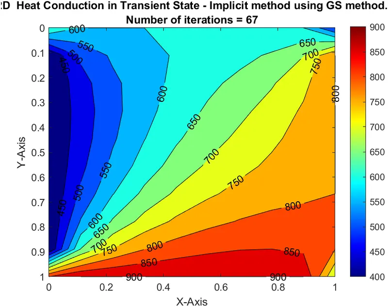
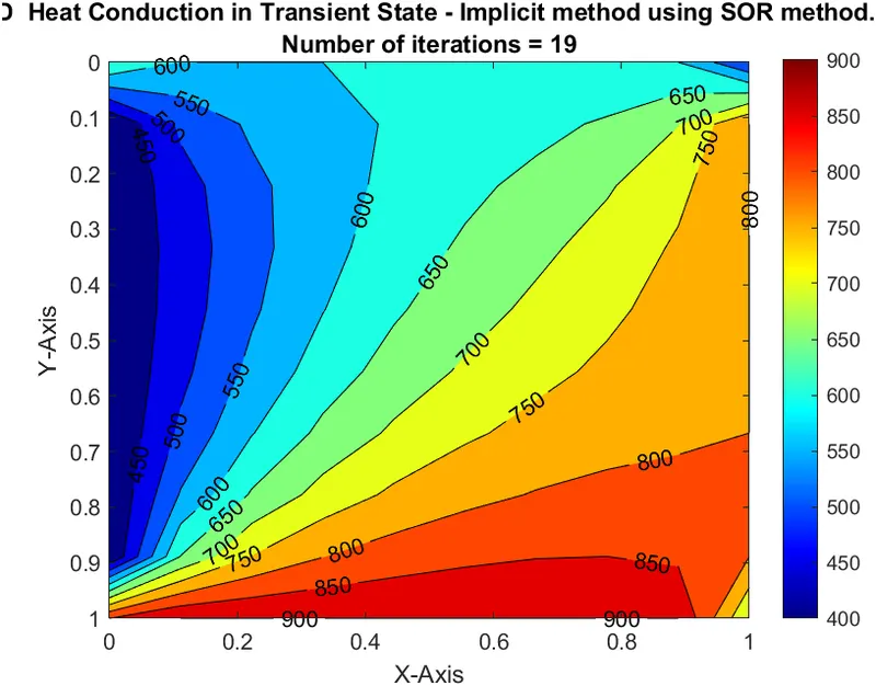
Resuts:
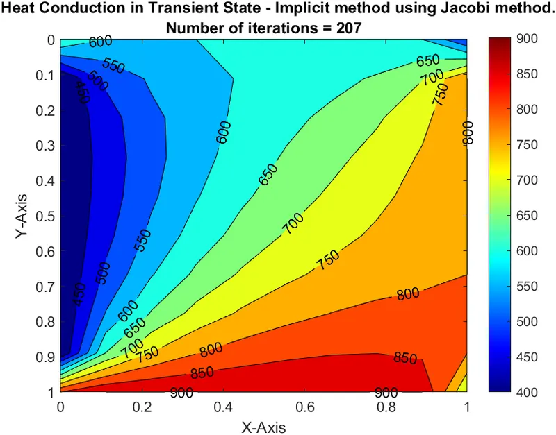
2D Transient state heat conduction (Explicit):
The 2D heat conduction equation in the transient state is as follows:
`(∂T)/(∂t) = α((del^2T)/(delx^2))+((del^2T)/(dely^2))`
Where, `alpha` is the thermal diffusivity.
if we discretize the above equation using Central Difference Method Explicitly, we get
`(T_P^(n+1))=(T_P^n)-αdeltat[((T_(R)-2T_(P)+T_(L))/(deltax^2))+((T_(T)-2T_(P)+T_(B))/(deltay^2))]^(n)`
if we simply further we get
`(T_P^(n+1))= (T_P^n + k1(T_(R)-2T_P+T_(L))^(n) + k2(T_(T)-2T_P+T_(B))^(n))`
where,
`k1 = alpha((deltat)/(deltax^2)) and k2 = alpha((deltat)/(deltay^2))`
The following code is the MATLAB code to solve for the 2D Transient/Unsteady-state heat conduction in the Explicit method.
close all
clear all
clc

%Solving the Transient state 2D heat conduction (EXPLICIT SCHEME)

%Input Parameters
%Number of grid points
nx = 10;
ny = nx;

x = linspace(0,1,nx);
y = linspace(0,1,ny);

dx = x(2) - x(1);
dy = dx;

%No of Time Steps
nt = 1500;
dt = 1e-3;

%Absolute error criteria > tolerance
error = 9e9;
tolerance = 1e-4;

%Defining Boundary conditions
T_L = 400;
T_T = 600;
T_R = 800;
T_B = 900;

T = 300*ones(nx,ny);

T(2:ny - 1, 1)  = T_L;
T(2:ny - 1, nx) = T_R;
T(1, 2:nx - 1)  = T_T;
T(ny, 2:nx - 1) = T_B;

%Calculating Average temperature at corners

T(1,ny) = (T_T + T_L)/2;
T(nx,1) = (T_R + T_B)/2;
T(nx,ny) = (T_T + T_R)/2;
T(1,1) = (T_L + T_B)/2;

%Assigning orginal values to T
T_intial = T;
T_old = T;

%Thermal Diffusivity Alpha
Alpha = 1.1;

%Calculation of 2D steady heat conduction EQUATION by Successive over-relaxation method
iterative_solver = 1;
k1 = Alpha*(dt/(dx^2));
k2 = Alpha*(dt/(dy^2));


if iterative_solver == 1
    Transient_Explicit = 1;
    for k = 1:nt
        error = 9e9;

        while(error > tolerance)

            for i = 2:nx - 1

                for j = 2:ny - 1
                    Term_1 = T_old(i,j);

                    Term_2 = k1*(T_old(i+1,j) - 2*T_old(i,j) + (T_old(i-1,j)));

                    Term_3 = k2*(T_old(i,j+1) - 2*T_old(i,j) + T_old(i,j-1));

                    T(i,j) = Term_1 + Term_2 + Term_3;
                end

            end

            error = max(max(abs(T_old - T)));
            T_old = T;
            Transient_Explicit = Transient_Explicit + 1;

        end
    end
end

%Plotting
figure(1)
contourf(x,y,T)
clabel(contourf(x,y,T))
colorbar
colormap(jet)
set(gca, 'ydir', 'reverse')

xlabel('X-Axis')
ylabel('Y-Axis')
title(sprintf('No. of Transient Iterations(EXPLICIT) = %d', Transient_Explicit));
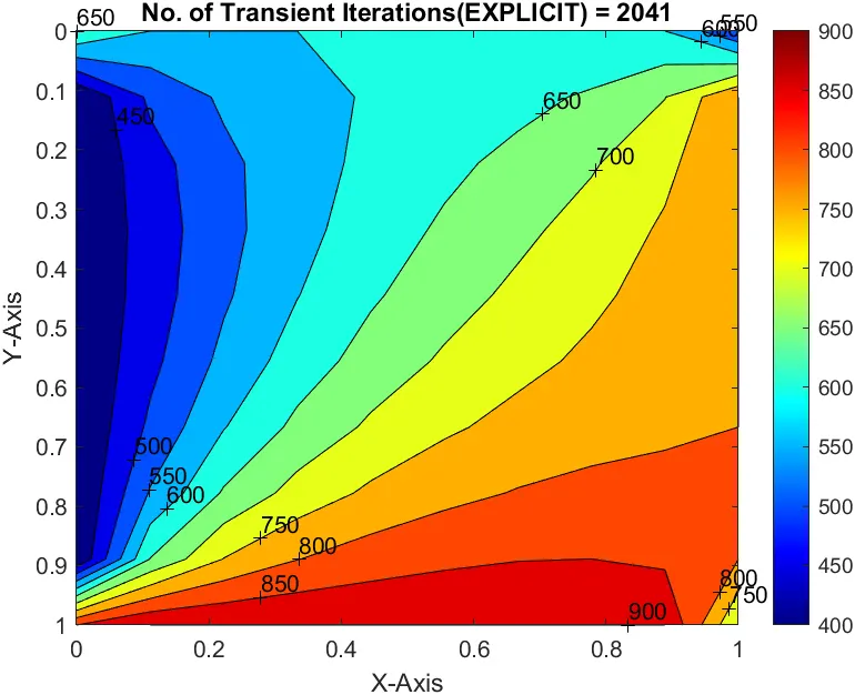
Results:
Conclusion:
From the above outputs of various methods & comparing their No. of iterations, we can conclude that
1. Jacobi > Gauss-seidel > Successive over-relaxation according to the No. of iterations computed for all iterative methods & different schemes.
2.SOR iteration method is the most effective iteration method as it took least No. of iterations for coverging solutions in both the schemes (EXPLICIT & IMPLICIT) compared to Jacobi & Gauss-siedel due to the relaxation factor (Alpha).
3. Explicit which is a direct scheme and which is conditionally stable attains the convergence at 2041 iterations with no of time steps taken as 1500. The iterations decreases as the time steps decreases. this shows that the no of iterations is directly proportional to the vallues of time step.