Matlab Program for solving and generating PV diagram plot of an Otto Cycle.

%this program is a system of equation as a function that accepts multiple input arguments: bore dia of the cyl, stroke length, connecting_rod length, compression ratio Cr, Start_crank angle and End_crank angle.


function [V] = Engine_kinematics(bore, stroke, con_rod, Cr, Start_crank, End_crank )

%Engine Geometric variables(Cr = comp. ratio, a = crank radius, R = ratio of con_rod/a)
a = con_rod/2;
R = con_rod/a;


%variables like Swept and clearance Volume can be computed from the
%relation

V_s = (pi/4)*bore^2*stroke;
V_c = V_s/(Cr-1);

%Angle of the Crank (theta)
theta = linspace(Start_crank, End_crank,100);

%Variables that determine the change in volume
term1 = 0.5*(Cr-1);
term2 = R + 1 - cosd(theta);
term3 = (R^2 - sind(theta).^2).^0.5;

%Total volume

V = (1 + term1 * (term2 - term3)).*V_c;
end

clear all
close all
clc

%program for plotting PV Diagram and Calculate Thermal Efficiency of the Engine

%Inputs for the calculation (Temperature at Point 3 and Ratio of Specific heat capacity Gamma)
T3 = 2300;
gamma = 1.4;

%Engine Geometric parameter variables
bore = 0.1;
stroke = 0.1;
con_rod = 0.15;
Cr = 12;

%state variables at point 1 (pressure N and temp K)
p1 = 101325;
T1 = 500;

%calculation for Swept volume V_s and Clearance volume V_c

V_s = (pi/4)*bore^2*stroke;
V_c = V_s/(Cr-1);

%therefore Volume at point 1 & 2 can be computed as
%V1 intial volume which is total volume of the cylinder
%V2 volume after compression, where compressed air fuel mixture is present.

V1 = V_s + V_c
V2 = V_c

%state variables at point 2 (pressure N and temp K) can be computed from the relation

%p1*V1^gamma = p2*V2^gamma | p2 = p1*(V1/V2)^gamma
% since Cr = V1/V2
% p2 = p1*Cr^gamma

p2 = p1*Cr^gamma;

%to compute the temperature at point 2, we use Ideal gas law
% p1*V1/T1 = p2*V2/T2
% T2 = p2*V2*T1/(p1*V1)

T2 = p2*V2*T1/(p1*V1)

%Determine the constant (p*V^gamma)
constant_c = p1*V1^gamma;

%volume and pressure during Compression process
%calling the function Engine_kinematics

V_compression = Engine_kinematics(bore,stroke,con_rod,Cr,180,0);

P_compression = constant_c./V_compression.^gamma;


%state variables at point 3
%since isentropic heat addition happens at constant volume, volume at point
%2 and 3 are constant/same, therefore

V3 = V2

%state variable at point 3 (pressure N )can be computed from Ideal Gas law
%p2V2/T2 = p3V3/T3

p3 = p2*T3/T2

%Determine the constant (p*V^gamma)
constant_c = p3*V3^gamma;

%volume and pressure during Expansion process
%calling the function Engine_kinematics

V_expansion = Engine_kinematics(bore,stroke,con_rod,Cr,0,180);

P_expansion = constant_c./V_expansion.^gamma;

%state variable at point 4
%since isentropic heat rejection happens at constant volume, volume at point
%4 and 1 are constant/same, therefore

V4 = V1

%pressure and temperature at point 4 can be computed from 
% p3*V3^gamma = p4*V4^gamma | p4 = p3*(V3/V4)^gamma

p4 = p3*(V3/V4)^gamma

%through Ideal gas equation temperature at point 4 is

T4 = p4*V4*T1/(p1*V1);

%The air-standard Otto cycle thermal efficiency is a function of compression ratio Cr and Gamma;
%The Thermal efficiency of the Air standard Otto Cycle is
%n_th = 1 - (T4-T1)/(T3-T2)
%n_otto = 1 - (V2/V1)^(gamma-1)
%n_otto = 1 - 1/(Cr^(gamma-1))

n_otto = 1 - 1/(Cr^(gamma-1));

%verifiying n_otto result
n_th = 1 - (T4-T1)/(T3-T2);

disp('Thermal_Efficiency of the Engine is');
disp(n_otto);
disp(n_th);

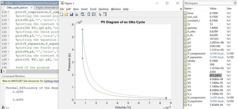
%plotting
figure(1)
hold on

title('PV Diagram of an Otto Cycle');
xlabel('Volume (V)');
ylabel('Pressure (p)');

%plotting the first point in the graph
plot(V1,p1,'*','color','r');
%plotting the compression curve in the graph
plot(V_compression,P_compression);
%plotting the second point in the graph
plot(V2,p2,'*','color','r');
%plotting the constant volume heat addition curve/line in the graph
plot([V2 V3],[p2 p3],'color','b');
%plotting the third point in the graph
plot(V3,p3,'*','color','r');
%plotting the expansion curve in the graph
plot(V_expansion,P_expansion);
%plotting the fourth point in the graph
plot(V4,p4,'*','color','r');
%plotting the constant volume heat rejection curve/line in the graph
plot([V1 V4],[p1 p4],'color','b');

%end of the program