Week 5.1 - Mid term project - Solving the steady and unsteady 2D heat conduction problem
MAIN PROGRAM FOR STEADY STATE ANALYSIS:
clear all
close all
clc

% Steady state analysis

n = 50; % number of grid points
x = linspace(0,1,n);
dx = x(2)-x(1);
dy = dx;
y = linspace(0,1,n);

T = 298*ones(n,n); % initial temperature condition
T(:,1) = 400; % K ,temperature left boundary condition
T(end,:) = 600; % K ,temperature top boundary condition
T(:,end) = 800; % K ,temperature right boundary condition
T(1,:) = 900; % K ,temperature bottom boundary condition

tol = 1e-4; % absolute error criteria
Told1 = T; Told2 = T; Told3 = T;
T1 = T; T2 = T; T3 = T;

% method: 1.Jacobi Method, 2.Gauss Seidel Method, 3.Successive Over
% Relaxation Method (SOR)


for method = 1:3

% jacobi method
if method == 1

    jac_error = 9e9; % initial value of error
    jacobi_iter = 0;
   tic
    while jac_error>tol
        jacobi_iter = jacobi_iter + 1;
        for i = 2:(n-1)
            for j = 2:(n-1)
                T1(i,j) = (Told1(i-1,j) + Told1(i+1,j) + Told1(i,j-1) + Told1(i,j+1))/4;
            end
        end
        jac_error = max(max(abs(T1-Told1)));
        Told1 = T1;

    end
    analysis_time1 = toc
        figure(1)
        contourf(x,y,T1,'Showtext','on')
        colormap(jet)
        colorbar
        xlabel('X axis')
        ylabel('Y axis')
        title(sprintf('2D Steady State Analysis (Jacobi Method) \nTemperature Distribution over a plate \nNumber of iterations = %d \nAnalysis time = %f seconds',jacobi_iter,analysis_time1))
        pause(0.02)

% gauss seidel method

elseif method == 2
    gauss_error = 9e9; % initial value of error
    gauss_iter = 0;
    tic
    while gauss_error>tol
        gauss_iter = gauss_iter + 1;
        for i = 2:(n-1)
            for j = 2:(n-1)
                T2(i,j) = (T2(i-1,j) + Told2(i+1,j) + T2(i,j-1) + Told2(i,j+1))/4;
            end

        end
        gauss_error = max(max(abs(T2-Told2)));
        Told2 = T2;
    end
    analysis_time2 = toc
        figure(2)
        contourf(x,y,T2,'Showtext','on')
        colormap(jet)
        colorbar
        xlabel('X axis')
        ylabel('Y axis')
        title(sprintf('2D Steady State Analysis (Gauss Seidel Method) \nTemperature Distribution over a plate \nNumber of iterations = %d \nAnalysis time = %f seconds',gauss_iter,analysis_time2))
        pause(0.02)

% SOR method

w = 2/(1+sin(pi*dx)); % relaxation parameter

elseif method == 3
    sor_error = 9e9; % initial value of error
    sor_iter = 0;
    tic
    while sor_error>tol
        sor_iter = sor_iter + 1;
        for i = 2:(n-1)
            for j = 2:(n-1)
                T3(i,j) = (1-w)*T3(i,j) + w*(T3(i-1,j) + Told3(i+1,j) + T3(i,j-1) + Told3(i,j+1))/4;
            end
        end
        sor_error = max(max(abs(Told3-T3)));
        Told3 = T3;
    end
    analysis_time3 = toc
        figure(3)
        contourf(x,y,T3,'Showtext','on')
        colormap(jet)
        colorbar
        xlabel('X axis')
        ylabel('Y axis')
        title(sprintf('2D Steady State Analysis (SOR Method) \nTemperature Distribution over a plate \nNumber of iterations = %d \nAnalysis time = %f seconds',sor_iter,analysis_time3))
        pause(0.02)
end
end
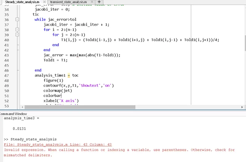
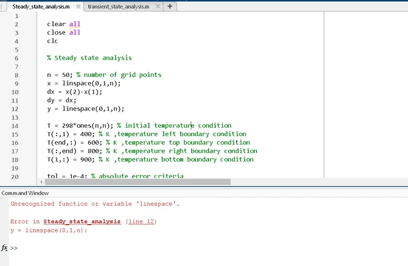
ERRORS FACING:
REPORT:
2D Steady state heat condution equation: (∂^2T/∂x^2)+(∂^2T/∂y^2)=0
* First we have to descritize the 2D steady state heat conduction equation, so that it can be solved numerically in matlab. After descritizing the equation we can solve the equation by three different iteration techniques. These are Jacobi method, Gauss Seidel method and Successive over relaxation method.
* First we define the number of grid points n=50, number of grid points in x direction is equal to the number of grid points in y direction. The metal plate is a thin square plate of size 1 m. After this we define the grit size dx and dy.
* Then we deifne the initial temperature condition to 298 kelvin accross entire nxn meshgrid, by using 'ones' command. And then we define the boundary temperature conditions according to the values given to us. Absoulte error criterio is equal to 1e-4, the error in the solution is compared after each iterations with absolute error criterio and if it is more than the absolute error, then the iterations keeps on going until the value of error is less than the absolute error criteria.
* Jacobi iteration method
Formula used:
T^n+1(i,j)=(T^n(i-1,j)+T^n(i+1,j)+T^n(i,j-1)+T^n(i,j+1))/4
* The above formula is used to calculate the value of T at time interval 'n+1'. In the above formula the RHS is assumed to have some intitial value, so the T at 'n+1' is assumed. Then for the first value fo i,j the value of T at 'n+1' is calculated. After first iteration the difference between the calculated value of T and previously assumed value T is calculated. If it more than the absolute error criteria or tolerance value, then the iteration keeps on going until the difference is less than the tolarance. Told value keep on uptading after each iteration inside the convergence loop.
* Gauss seidel method
Formula used:
T^n+1(i,j)=(T^n(i-1,j)+T^n(i+1,j)+T^n+1(i,j-1)+T^n(i,j+1))/4
* The above formula is similar to the jacobi method but when the first iteration is run to calculate the value fo T at a node, then this updated value of T is used to calculate the value at the next node. This technique decreases the convergence time.
* Successive over relaxation method
Formula used:
T^n+1(i,j)=(1-ω)T^n+1(i,j)+ω ((T^n+1(i,j-1)+T^n(i+1,j)+T^n(i,j+1))/4
* This technique can be applied to both jacobi and gauss Seidel method, in this method a relaxation parameter 'w' is used which over estimates the value and leads to an increase value in T for each iteration, in this way the convergence is achived much faster than the above two methods.
Formula for relxation parameter: ω = 2/(1+sin(pi.dx))
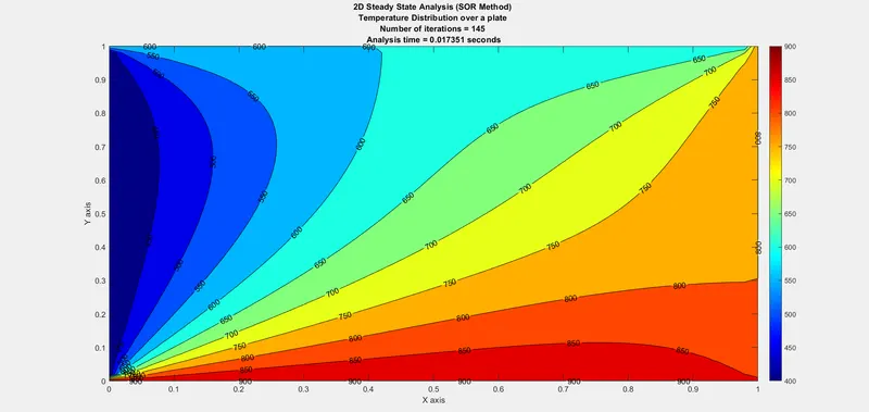
* We used 'tic' and 'toc' command to calculate the time of convergence for each of the three iteration method. After each convergence loop we plot the result on a contour plot between x,y,T. Contour plot visulises the temperature distribution over the plate and also gives us the number of iterations and time needed for convergence.
OUTPUT:
Figure 1:
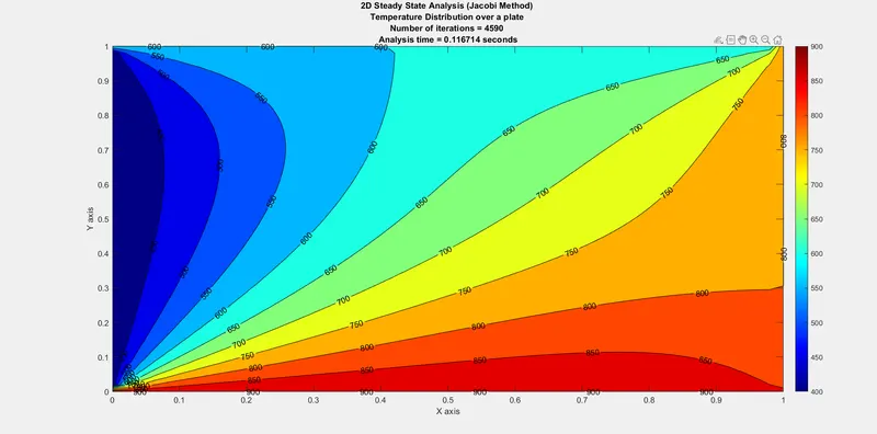
Figure 2:
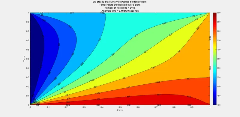
Figure 3:
EXPLANATION :
* The three graphs above shows the temperature distribution over a thin metal plate. And also displays the number of iterations and analysis time.
* From the above graphs we can say that jacobi method has maximum number of iterations than the rest of the methods. And convergence time is also more than other methds.
* Number of iterations and convergence time for Gauss Seidel method is less than jacobi method but more than SOR method.
* The successive over relaxation method has least number of iterations and it took least time for convergence.
* In 2D steady state analysis SOR method is fastest.
MAIN PROGRAM FOR TRANSIENT STATE ANALYSIS:
clear all
close all
clc

% transient heat conduction

n = 50; % number of grid points
x = linspace(0,1,n);
dx = x(2) - x(1);
dy = dx;
y = linspace(0,1,n);
total_time = 10;
dt = 0.01;
total_time_steps = total_time/dt;

T = 298*ones(n,n); % initial temperature condition
T(:,1) = 400; % K ,temperature left boundary condition
T(end,:) = 600; % K ,temperature top boundary condition
T(:,end) = 800; % K ,temperature right boundary condition
T(1,:) = 900; % K ,temperature bottom boundary condition
% defining the corner temperature for smoother graph
T(1,1) = 500; % k top left boundary condition
T(n,1) = 650; % k bottom left boundary condition
T(1,n) = 700; % k top right boundary condition
T(n,n) = 850; % k bottom right boundary condition

tol = 1e-4;
Alpha = 0.002; % thermal diffusivity
k = Alpha*dt/(dx^2);
CFL = Alpha*dt/(dx^2);

Told1 = T; Told2 = T; Told3 = T; Told4 = T;
T1 = T; T2 = T; T3 = T; T4 = T;
T_time1  = T; T_time2 = T; T_time3 = T; T_time4 = T; % for time loop

% 1.transient explicit, 2.transient implicit jacobi, 3.transient implicit gauss seidel, 4.transient
% implicit SOR

for method = 1:4

    % 1.transient explicit

  if method ==1
       cycle = 0;
        tic
        for t = 1:total_time_steps
            for i = 2:(n-1)
                for j = 2:(n-1)
                    T1(i,j) = Told1(i,j) + k*(Told1(i-1,j) + Told1(i+1,j) + Told1(i,j-1) + Told1(i,j+1)-4*Told1(i,j));
                end
            end
            Told1 = T1;
            cycle = cycle + 1;
        end
        convergence_time1 = toc;
        figure(1)
        contourf(x,y,T1,'Showtext','on')
        colormap(jet)
        colorbar
        xlabel('X axis')
        ylabel('Y axis')
        title(sprintf('2D Transient State Analysis (Explicit Method) \nTemperature Distribution over a plate \nNumber of cycles = %d \nTime for convergence = %f seconds',cycle,convergence_time1))
        pause(0.02)


   % 2.transient implicit jacobi
elseif method == 2
       tic
       for t = 1:total_time_steps
           jacobi_error = 9e9;
           jacobi_iter = 0;
           while (jacobi_error>tol)
               jacobi_iter = jacobi_iter + 1;
               for i = 2:(n-1)
                   for j = 2:(n-1)
                       T2(i,j) = T_time2(i,j)/(1+4*k) + (k/(1+4*k))*(Told2(i-1,j) + Told2(i+1,j) + Told2(i,j-1) + Told2(i,j+1));
                   end
               end
               jacobi_error = max(max(abs(T2-Told2)));
               Told2 = T2;
           end
           T_time2 = T2;
       end
        convergence_time2 = toc;
        figure(2)
        contourf(x,y,T2,'Showtext','on')
        colormap(jet)
        colorbar
        xlabel('X axis')
        ylabel('Y axis')
        title(sprintf('2D Transient State Analysis (Implicit Jacobi Method) \nTemperature Distribution over a plate \nNumber of iterations = %d \nTime for convergence = %f seconds',jacobi_iter,convergence_time2))
        pause(0.02)

   % 3.transient implicit gauss seidel
elseif method == 3
       tic
       for t = 1:total_time_steps
           GS_error = 9e9;
           GS_iter = 0;
           while(GS_error>tol)
               GS_iter = GS_iter + 1;
               for i = 2:(n-1)
                   for j = 2:(n-1)
                       T3(i,j) = T_time3(i,j)/(1+4*k) + (k/(1+4*k))*(T3(i-1,j) + Told3(i+1,j) + T3(i,j-1) + Told3(i,j+1));
                   end
               end
               GS_error = max(max(abs(Told3-T3)));
               Told3 = T3;
           end
           T_time3 = T3;
       end
        convergence_time3 = toc;
        figure(3)
        contourf(x,y,T3,'Showtext','on')
        colormap(jet)
        colorbar
        xlabel('X axis')
        ylabel('Y axis')
        title(sprintf('2D Transient State Analysis (Implicit Gauss Seidel Method) \nTemperature Distribution over a plate \nNumber of iterations = %d \nTime for convergence = %f seconds',GS_iter,convergence_time3))
        pause(0.02)


  % 4.transient implicit SOR
  elseif method == 4

      w = 2/(1+sin(pi*dx)); % relaxation parameter

      tic
      for t = 1:total_time_steps
          SOR_error = 9e9;
          SOR_iter = 0;
          while (SOR_error>tol)
              SOR_iter = SOR_iter + 1;
              for i = 2:(n-1)
                  for j = 2:(n-1)
                      T4(i,j) =(1-w)*Told4(i,j) + w*(T_time4(i,j))/(1+4*k) + w*(k/(1+4*k))*(T4(i-1,j) + Told4(i+1,j) + T4(i,j-1) + Told4(i,j+1));
                  end
              end
              SOR_error = max(max(abs(Told4-T4)));
              Told4 = T4;
          end
          T_time4 = T4;
      end
        convergence_time4 = toc;
        figure(4)
        contourf(x,y,T4,'Showtext','on')
        colormap(jet)
        colorbar
        xlabel('X axis')
        ylabel('Y axis')
        title(sprintf('2D Transient State Analysis (Implicit SOR Method) \nTemperature Distribution over a plate \nNumber of iterations = %d \nTime for convergence = %f seconds',SOR_iter,convergence_time4))
        pause(0.02)

  end

end
REPORT:
2D Transient State heat conduction equation:
∂T/∂t=α(∂^2T/∂x^2)+(∂^2T/∂y^2)
* We have to descritize the 2D Transient state heat conduction equation, so that it can be solved numerically in matlab. After descritizing the equation we can solve the equation by explicit and implicit method. In implicit method we can use three different iteration techniques, these are Jacobi method, Gauss Seidel method and Successive over relaxation method.
* First we define the number of grid points n=50, number of grid points in x direction is equal to the number of grid points in y direction. The metal plate is a thin square plate of size 1 m. After this we define the grit size dx and dy.
* Then we deifne the initial temperature condition to 298 kelvin accross entire nxn meshgrid, by using 'ones' command. And then we define the boundary temperature conditions according to the values given to us. Absoulte error criterio is equal to 1e-4, the error in the solution is compared after each iterations with absolute error criterio and if it is more than the absolute error, then the iterations keeps on going until the value of error is less than the absolute error criteria.
* As this is a Transient state analysis, there is a time derivative in the equation, for this we have to define a time loop which will run for the defined number of time steps. We have to define the value of total time for the simulation, time step (dt) and total number of time steps. We also have to take a value for thermal diffusivity alpha = 0.002.
* Explicit method
K=α(dt/dx^2)
Formula for explicit method:
T^n+1(i,j)=(T^n(i,j)K(T^n(i-1,j)+T^n(i+1,j)+T^n+1(i,j-1)+T^n(i,j+1)-4.T^n(i,j)
The above formula is defined in a time loop. The loop runs for 1000 time steps. Told is updated in each time loop. The initial value of RHS is assumed which gives us the assumed value of T at 'n+1' time interval. For next value of i,j ,T is calculated at the next node. The equations converges in 1000 time steps to give the solution.
In explicit scheme there is simple updating of old value take place and the solution does not depend upon other value at the current level. While implicit scheme contains the information at the current level which requires solution of simaultaneous equations.
* Implicit Jacobi method
Formula for implicit Jacobi method:
T^n+1(i,j)=(T time (i, j)/1+4k)+(k/1+4k).(T^n(i-1,j)+T^n(i+1,j)+T^n(i,j-1)+T^n(i,j+1))
The above formula is defined in a convergence loop, which itself is defined in a time loop. Told is updated in convergence loop and T_time values are updated in time loop. The initial values are assumed and the first iteration is done to calculate the T at 'n+1' time interval at the next node. After each convergence loop the difference between previous value of T and calculated value of T is calculated. The error is compared to the tolerance value, the iterations keeps on going until the error value is less than tolarance.
* Implicit Gauss Seidel method
Fromula for implicit Gauss Seidel method:
T^n+1(i,j)=(T time (i, j)/1+4k)+(k/1+4k).(T^n+1(i-1,j)+T^n(i+1,j)+T^n+1(i,j-1)+T^n(i,j+1))
The above formula is defined in a convergence loop, which itself is defined in a time loop. Told is updated in convergence loop and T_time values are updated in time loop. The above formula is similar to implicit jacobi method, except, when the first iteration is done to calculate the value of T, this updated value of T is used to calculate value of T at next node. The error is compared after each convergence loop.
* Implicit Successive over relaxation (SOR) method
Formula for implicit SOR method:
T^n+1(i,j)=(1-ω)T^n+1(i,j)+ω(T time (i, j)/1+4k)+(k/1+4k).(T^n+1(i-1,j)+T^n(i+1,j)+T^n+1(i,j-1)+T^n(i,j+1))
The above formula is defined in a convergence loop, which itself is defined in a time loop. Told is updated in convergence loop and T_time values are updated in time loop. SOR method contains relaxation parameter which causes more increment of T for each iterations. The error is compared after each convergence loop.
Formula for relxation parameter: ω = 2/(1+sin(pi.dx))
We used 'tic' and 'toc' command to calculate the time of convergence for explicit and implicit method. After each time loop we plot the result on a contour plot between x,y,T. Contour plot visulises the temperature distribution over the plate and also gives us the number of iterations and time needed for convergence.
OUTPUTS:
Figure 1:
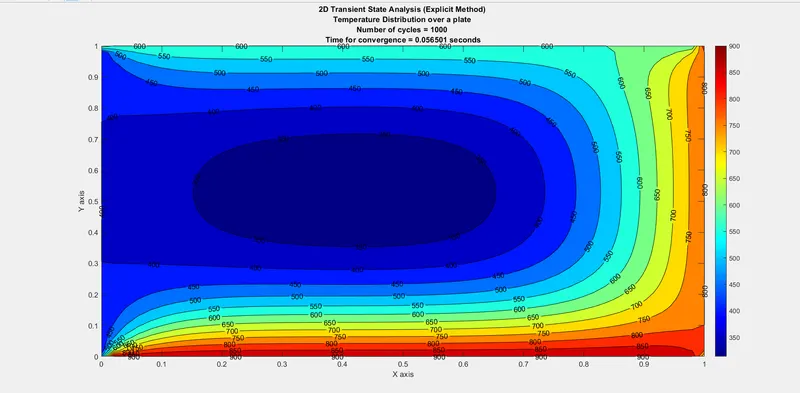
Figure 2:
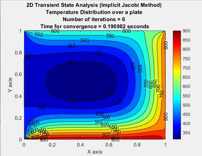
Figure 3:
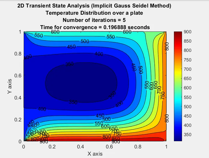
Figure 4:
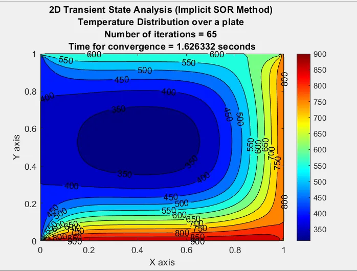
EXPLANATIONS:
* From the above graphs it is clear that explicit method is faster than implicit method to solve 2D transient state heat conduction equation.
* Among implicit method the Guass seidel method took least time for convergence.
* Jacobi method took less time for convergence than SOR but took more time than Gauss seidel method.
* 9Maxmum time for convergence was taken by SOR method.
* In 2D transient state analysis, while solving implicitly the number of Jacobi, Gauss Seidel and SOR iterations are less than the steady state analysis. But the time of convergence is more, this happens because here thermal diffusivity (Alpha) and time derivative is taken into consideration.