Week 5.1 - Mid term project - Solving the steady and unsteady 2D heat conduction problem
Problem Statement:
Solving for 2D heat conduction equation for steady and unsteady state by explicit and implicit method with given boundary conditions.
Using implicit method
Solve using different iterative solvers i.e., Jacobi, Gauss seidal, and Successive overrelaxation for both steady and transient state heat conduction equation.
The accuracy of the solution obtained in both explicit and implicit methods should be by the tolerance value mentioned.
Boundary conditions:
Top Boundary = 600 K
Bottom Boundary = 900 K
Left Boundary = 400 K
Right Boundary = 800 K
Tolerance value => error = 1e-4.
Formulas:
To solve for dependent variable iterative solvers are used. Iterative solvers used are
1. Jacobi iterative solver
2. Gauss seidal iterative solver
3. Successive over-relaxation iterative solver.
2D Heat Conduction Equation
∂T∂t=α⋅(∂2T∂x2+∂2T∂y2)∂T∂t=α⋅(∂2T∂x2+∂2T∂y2)
T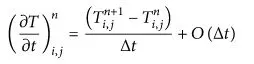
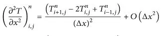
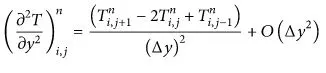

where n is the current time step and n+1 is the next time step.
I,i+1 are the neighboring points in the x direction, and j,j+1 are the neighboring points in the y direction.
△x△x is grid spacing in the x direction. △y△y is grid spacing in the y direction.
Iterative Solver:
1. Jacobi iterative solver:
In this method, the temperature at n+1th iteration is found using old values of the temperature defined at nth iterations. Using the approximation obtained iterations procedure it continued until the desired accuracy of the solution is obtained.
2. Gauss Seidel iterative solver:
In this type of iterative solver, the temperature at n+1 iterations uses values of n+1 iterations that have already been computed. In this way, old approximated values are overwritten with new approximate values for the iterations performed. Unlike Jacobi, Gauss seidel requires one storage vector which can be overwritten with each computation. This helps the solution to cover faster than the Jacobi method.
3. Successive over-relaxation iterative solver.
In this type of iterative solver relaxation factor is used which helps in increasing the convergence rate. It goes by the formula
Tn+1=Tn⋅(1−ω)+ω⋅T(GS)orT(jacobi)Tn+1=Tn⋅(1-ω)+ω⋅T(GS)orT(jacobi)
where ωω is the relaxation factor. Its range is from 0<ωω<2
when ωω is between 0-1 it is called under relaxed state.
This condition is used when the temperature gradient is high and due to this condition, the time step does not overshoot and helps to converge at a faster rate.
when ωω is between 1-2 it is called an over the relaxed state.
This condition is used when the temperature gradient is low and due to this condition, larger time steps are used to obtain the steady state i.e., for the values to converge at a faster rate.
TnTn is the value of temperature for previous iterations
T(GS) or T(Jacobi) is the temperature of value for n+1th iteration using gauss seidal or Jacobi iterative solver.
Steady State 2D Heat Conduction Equation :
A steady state is where the fluid properties do not change over time.
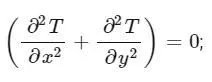
From the 2D heat conduction equation since the system is in a steady state time derivative is zero and diffusivity is constant.

Hence the equation for the steady state as:-
Discretization for Steady State:

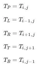
Solving for T(i,j), we get

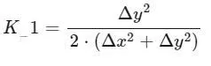 ,
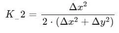
, 
Solving the 2D Steady Heat Conduction equation implicitly.
Formula for Jacobi iterative solver:-

The formula for Gauss-Seidel Iterative Solver:-
(Tp)n+1=K1(TL+Tr)n+1+K2(TT+TB)n+1(Tp)n+1=K1(TL+Tr)n+1+K2(TT+TB)n+1
The formula for Successive over-relaxation iterative solver:-

Transient state:
The unsteady state is where the fluid properties change over time.
The formula for the 2D transient heat conduction equation is :
∂T∂t=α⋅(∂2T∂x2+∂2T∂y2)∂T∂t=α⋅(∂2T∂x2+∂2T∂y2)
Discretization for Unsteady State heat conduction equation:-

Solving the 2D transient heat conduction equation explicitly we get,
Tn+1P=(1−2⋅K1−2⋅K2)⋅TnP+K1(TL+TR)n+K2(TT+TB)nTPn+1=(1-2⋅K1-2⋅K2)⋅TPn+K1(TL+TR)n+K2(TT+TB)n
K1=α⋅△t△x2K1=α⋅△t△x2
K2=α⋅△t△y2K2=α⋅△t△y2
Stability Criteria:
K1+K2≤0.5K1+K2≤0.5 Stability criteria for 2D heat conduction equation when solving explicitly.
Solving for 2D Transient Heat Conduction equation implicitly we get,
Tn+1P=1K⋅[TnP+K1(TL+TR)n+1+K2(TT+TB)n+1]TPn+1=1K⋅[TPn+K1(TL+TR)n+1+K2(TT+TB)n+1]
K=1+2⋅K1+2⋅K2K=1+2⋅K1+2⋅K2
K1=α⋅△t△x2K1=α⋅△t△x2
K2=α⋅△t△y2K2=α⋅△t△y2
here n+1 is the next time step and n is the preceding time step.
Formula for jacobi iterative solver:-

The formula for Gauss said

The formula for Successive over relaxation

Matlab code:
Main code:
%Code to study the behavior of steady state and transient state analysis
%using the explicit and implicit methods.
clear all
close all
clc
%Defining the spatial domain
nx = 10;ny=10;
%Specifying length of the domain.
L=1;
%defining space domain
x = linspace(0,L,nx);
y = linspace(0,L,ny);
%grid size
dx = x(2)-x(1);
dy = y(2)-y(1);
%defining temperature
t = 300*ones (nx,ny);
% [t] = 300*meshgrid(x,y);
t(1:end,1)=400;%<-- left boundary
t(end,1:end)=900;%<-- bottom boundary
t(1,1:end)=600;%<-- top boundary
t(1:end,end)=800;%<-- right boundary
% Edge temperature
t(1,1)= (t(1,2)+t(2,1))/2;
t(end,1) = (t(end,2)+t((end-1),1))/2;
t(1,end)= (t (1,(end-1))+t(2,end))/2;
t(end,end)=(t((end-1),(end))+ t(end,(end-1)))/2;
%tolerance
tol=1e-4;
%Making a copy of the initial temperature matrix.
told=t;
t_pre=t;
%Coefficient obtained from the derivation for steady state equation
k = 2*(dx^2+dy^2)/(dx^2*dy^2);
%diffusivity co-efficient in the 2D heat conduction equation
alpha = 1.4;
% Calculation of time step
dt = (0.5)/((alpha/dx^2)+(alpha/dy^2));
% Co-efficient multiplied for x diffuse term
k1 = dt*alpha/dx^2;
% Co-efficient multiplied for y diffuse term
k2 = dt*alpha/dy^2;
%relaxation factor for successive over-relaxation factor for steady state
%heat conduction.
a = 1.5;
%relaxation factor for Successive over-relaxation factor for transient heat
%conduction
a1 = 1.15;
%Function to calculate the temperature of Steady-state using Jacobi iterative solver
[error_j,iter1] = jacobi(nx,ny,t,told,k,dx,dy,tol);
%Function to calculate the temperature of Steady-state using Gauss-Seidel iterative solver
[error_gs,iter2] = gs(nx,ny,t,told,k,dx,dy,tol);
%Function to calculate the temperature Steady state using Successive over-relaxation iterative solver
[error_sor_gs,iter3] = sor_gs(nx,ny,t,told,k,dx,dy,tol,a);
%Function to calculate the temperature of Transient heat conduction explicitly
[error_dt,iter_dt]=transient_heat_conduction(nx,ny,k1,k2,told,t,tol);
%Function to calculate the temperature of Unsteady state using Jacobi iterative solver
[error_jac,iter_jac]=transient_heat_conduction_jacobi(nx,ny,k1,k2,told,t,tol,t_pre);
%Function to calculate the temperature of Unsteady state using Gauss-Seidel iterative solver
[error_gs_imp,iter_gs_imp]=transient_heat_conduction_gs(nx,ny,k1,k2,told,t,tol,t_pre);
%Function to calculate the temperature of Unsteady state using Successive over-relaxation iterative solver
[error_sor_gs_imp,iter_sor_gs_imp]=transient_heat_conduction_sor_gs(nx,ny,k1,k2,told,t,tol,t_pre,a1);
Function to calculate the temperature of Steady-state using Jacobi iterative solver:
%Function to calculate the temperature of Steady-state using Jacobi iterative solver
function [error_j,iter1] = jacobi(nx,ny,t,told,k,dx,dy,tol)
%defining iteration variable to store and display the number of
%iterations computed for the values to converge.
iter1 = 0;
% Dummy error value
error_j = 9e9;
%convergence loop
while (error_j>tol)
%Iteration loop
for i = 2:(nx-1)
for j = 2:(ny-1)
%Formula to calculate the temperature at each grid
%point
t(i,j)= (1/k)*(((told((i-1),j)+told((i+1),j))/dx^2)+((told(i,(j+1))+told(i,(j-1)))/dy^2));
end
end
%error for each iteration
error1 = abs(told-t);
error_j = max(error1,[],'all');
%updating the temperature values for the next iteration.
told = t;
%incrementing iter variable by 1 to display the no. of
%iterations taken for the solution to converge.
iter1 = iter1+1;
end
% Plot representing the converged results.
figure(1)
[C,h]=contourf(t);
%Labelling the plot here C represents the temperature values and h rotates the temperature values as it moves.
clabel(C,h);
axis ij;
title('number of iterations for Jacobi method for steady-state heat conduction',iter1);
end
Function to calculate the temperature of Steady-state using Gauss-Seidel iterative solver:
%Function to calculate the temperature of Steady-state using Gauss Seidel iterative solver
function [error_gs,iter2] = gs(nx,ny,t,told,k,dx,dy,tol)
% Dummy error value
error_gs = 9e9;
%defining iteration variable to store and display the number of
%iterations computed for the values to converge.
iter2 = 0;
%convergence loop
while (error_gs>tol)
%Iteration loop
for i = 2:(nx-1)
for j = 2:(ny-1)
%Formula to calculate the temperature at each grid
%point
t(i,j)= (1/k)*(((t((i-1),j)+t((i+1),j))/dx^2)+((t(i,(j+1))+t(i,(j-1)))/dy^2));
end
end
%error for each iteration
error1 = abs(told-t);
error_gs = max(error1,[],'all');
%updating the temperature values for the next iteration.
told = t;
%incrementing iter variable by 1 to display the no. of
%iterations taken for the solution to converge.
iter2 = iter2+1;
end
% Plot representing the converged results.
figure(2)
[C,h]=contourf(t);
%Labelling the plot here C represents the temperature values and h rotates the temperature values as it moves.
clabel(C,h);
axis ij;
title('Number of iterations for Gauss seidal method steady state heat conduction',iter2)
end
Function to calculate the temperature of Steady-state using Successive over-relaxation iterative solver:
%Function to calculate the temperature of Steady-state using Successive over-relaxation iterative solver
function [error_sor_gs,iter3] = sor_gs(nx,ny,t,told,k,dx,dy,tol,a)
%Dummy error value
error_sor_gs = 9e9;
%defining iteration variable to store and display the number of
%iterations computed for the values to converge.
iter3 = 0;
%Convergence loop
while (error_sor_gs>tol)
%iteration loop
for i = 2:(nx-1)
for j = 2:(ny-1)
%Formula to calculate the temperature at each grid
%point
t(i,j)= (1/k)*(((t((i-1),j)+told((i+1),j))/dx^2)+((told(i,(j+1))+t(i,(j-1)))/dy^2));
%Successive over relaxation Formula to calculate the
%temperature at each grid point.
t(i,j) = (told(i,j))*(1-a)+a*(t(i,j));
end
end
%error for each iteration
error1 = abs(told-t);
error_sor_gs = max(error1,[],'all');
%updating the temperature values for the next iteration.
told = t;
%incrementing iter variable by 1 to display the no. of
%iterations taken for the solution to converge.
iter3 = iter3+1;
end
% Plot representing the converged results.
figure(3)
[C,h]=contourf(t);
%Labelling the plot here C represents the temperature values and h rotates the temperature values as it moves.
clabel(C,h);
axis ij;
title('number of iterations for Successive over relaxation method for steady-state heat conduction', iter3)
end
Function to calculate the temperature of Unsteady state using the explicit method:
%Function to calculate the temperature of the Unsteady state using explicit
%method
function [error_dt,iter_dt]=transient_heat_conduction(nx,ny,k1,k2,told,t,tol)
%dummy error
error_dt = 9e9;
%defining iteration variable to store and display the number of
%iterations computed for the values to converge.
iter_dt =0;
%convergence loop
while (error_dt>tol)
%Iteration loop
for i = 2:nx-1
for j = 2:ny-1
H = told(i-1,j)-2*told(i,j)+told(i+1,j);%<-- This line represent temperature values in x direction
V = told(i,j-1)-2*told(i,j)+told(i,j+1);%<-- This line represent temperature values in y direction
%Formula to calculate the temperature at each grid
%point
t(i,j)= told(i,j)+k1*H+k2*V;
end
end
%error for each iteration
error1 = abs(told-t);
error_dt = max(error1,[],'all');
%updating the temperature values for the next iteration.
told = t;
%incrementing iter variable by 1 to display the no. of
%iterations taken for the solution to converge.
iter_dt = iter_dt+1;
end
%Plot representing the converged results.
figure(4)
[C,h]=contourf(t);
%Labelling the plot here C represents the temperature values and h rotates the temperature values as it moves.
clabel(C,h);
axis ij
title('Number of iterations using transient heat conduction explicitly',iter_dt);
end
Function to calculate the temperature in Unsteady state using Jacobi iterative solver:
%Function to calculate the temperature of Unsteady state using Jacobi
%iterative solver
function [error_jac,iter_jac]=transient_heat_conduction_jacobi(nx,ny,k1,k2,told,t,tol,t_pre)
% dummy error
error_jac=9e9;
error_f = 9e9;
%defining iteration variable to store and display the number of
%iterations computed for the values to converge.
iter_jac=0;
%While loop to stop iterations when the temperature values converge
%whle computing for different time steps.
while (error_f>tol)
%Convergence loop each time step
while (error_jac>tol)
%Iteration loop
for i = 2:nx-1
for j = 2:ny-1
%Co-efficient obtained while deriving for transient heat conduction equation
term1= (1+(2*k1)+(2*k2))^-1;
%k1 and k2 represent the cfl value for x and y
%domain respectively.
H = told(i-1,j)+told(i+1,j);%<-- This line represent temperature values in x direction
V = told(i,j-1)+told(i,j+1);%<-- This line represent temperature values in y direction
%Formula to calculate the temperature at each grid
%point
t(i,j)= (t_pre(i,j)*term1)+(term1*k1*H)+(term1*k2*V);
end
end
%error for each iteration
error1 = abs(told-t);
error_jac = max(error1,[],'all');
%updating the temperature values for the next iteration.
told = t;
%incrementing iter variable by 1 to display the no. of
%iterations taken for the solution to converge.
iter_jac = iter_jac+1;
end
% error defined to obtain the desired accuracy for the convergence rate.
error_f = max(max(abs(t_pre-t)));
t_pre = t;
%Reseting the error value for the convergence loop to compute for the
%next time step.
error_jac = 9e9;
end
%Plot representing the converged results.
figure(5)
[C,h]=contourf(t);
%Labelling the plot here C represents the temperature values and h rotates the temperature values as it moves.
clabel(C,h)
axis ij
title('Number of iterations for implicit Jacobi',iter_jac);
end
Function to calculate the Temperature in an Unsteady state using Gauss seidal iterative solver.
%Function to calculate the temperature of Unsteady state using gauss seidel
%iterative solver
function [error_gs_imp,iter_gs_imp]=transient_heat_conduction_gs(nx,ny,k1,k2,told,t,tol,t_pre)
%Definition of dummy error
error_f = 9e9;
error_gs_imp=9e9;
%defining iteration variable to store and display the number of
%iterations computed for the values to converge.
iter_gs_imp=0;
%While loop to stop iterations when the temperature values converge
%whle computing for different time steps.
while(error_f>tol)
%Convergence loop each time step
while (error_gs_imp>tol)
%Iteration loop
for i = 2:nx-1
for j = 2:ny-1
%Co-efficient obtained while deriving for transient heat conduction equation
term1= (1+(2*k1)+(2*k2))^-1;
%k1 and k2 represent the cfl value for x and y
%domain repectively.
H = t(i-1,j)+told(i+1,j);%<-- This line represent temperature values in x direction
V = t(i,j-1)+told(i,j+1);%<-- This line represent temperature values in y direction
%Formula to calculate the temperature at each grid
%point
t(i,j)= (t_pre(i,j)*term1)+(term1*k1*H)+(term1*k2*V);
end
end
%error for each iteration
error1 = abs(told-t);
error_gs_imp = max(error1,[],'all');
%updating the temperature values for the next iteration.
told = t;
%incrementing iter variable by 1 to display the no. of
%iterations taken for the solution to converge.
iter_gs_imp = iter_gs_imp+1;
end
% error defined to obtain the desired accuracy for the convergence rate.
error_f = max(max(abs(t_pre-t)));
%Updating the previous temperature values to computed values.
t_pre = t;
%Reseting the error value for the convergence loop to compute for the
%next time step.
error_gs_imp = 9e9;
end
%Plot representing the converged results.
figure(6)
[C,h]=contourf(t);
%Labelling the plot here C represents the temperature values and h rotates the temperature values as it moves.
clabel(C,h)
axis ij
title('Number of iterations for implicit Gauss seidal',iter_gs_imp);
end
Function to calculate the temperature in Unsteady state using a successive over-relaxation iterative solver
%Function to calculate the temperature of the Unsteady state using successive
%over relaxation iterative solver
function [error_sor_gs_imp,iter_sor_gs_imp]=transient_heat_conduction_sor_gs(nx,ny,k1,k2,told,t,tol,t_pre,a1)
%Definition of dummy error
error_f = 9e9;
error_sor_gs_imp = 9e9;
%defining iteration variable to store and display the number of
%iterations computed for the values to converge.
iter_sor_gs_imp =0;
%While loop to stop iterations when the temperature values converge
%whle computing for different time steps.
while (error_f>tol)
%Convergence loop each time step
while (error_sor_gs_imp>tol)
%Iteration loop
for i = 2:nx-1
for j = 2:ny-1
%Co-efficient obtained while deriving for transient heat conduction equation
term1= (1+(2*k1)+(2*k2))^-1;
H = t(i-1,j)+told(i+1,j);%<-- This line represent temperature values in x direction
V = t(i,j-1)+told(i,j+1);%<-- This line represent temperature values in y direction
%Formula to calculate the temperature at each grid
%point
t(i,j)= (t_pre(i,j)*term1)+(term1*k1*H)+(term1*k2*V);
%Successive over relaxation Formula to calculate the
%temperature at each grid point.
t(i,j)= (told(i,j))*(1-a1)+ a1*t(i,j);
end
end
%error for each iteration
error1 = abs(told-t);
error_sor_gs_imp = max(error1,[],'all');
%updating the temperature values for the next iteration.
told = t;
%incrementing iter variable by 1 to display the no. of
%iterations taken for the solution to converge.
iter_sor_gs_imp = iter_sor_gs_imp+1;
end
%error defined to obtain the desired accuracy for the convergence rate.
error_f = max(max(abs(t_pre-t)));
%Updating the previous temperature values to computed values.
t_pre = t;
%Reseting the error value for the convergence loop to compute for the
%next time step.
error_sor_gs_imp = 9e9;
end
%Plot representing the converged results.
figure(7)
[C,h]=contourf(t);
%Labelling the plot here C represents the temperature values and h rotates the temperature values as it moves.
clabel(C,h)
axis ij
title('Number of iteration for implicit SOR',iter_sor_gs_imp);
end
Results:
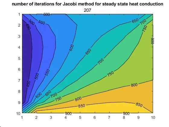
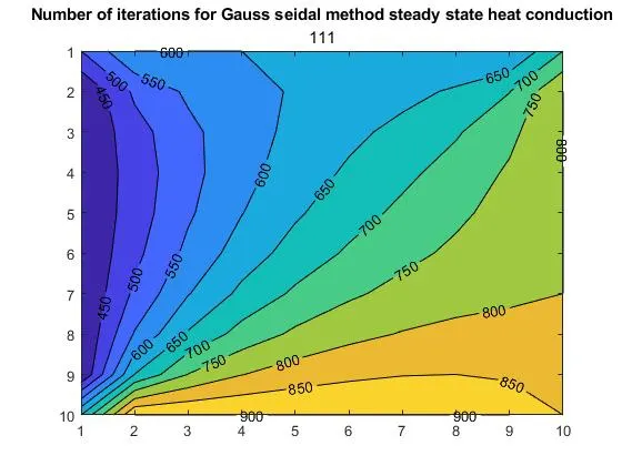
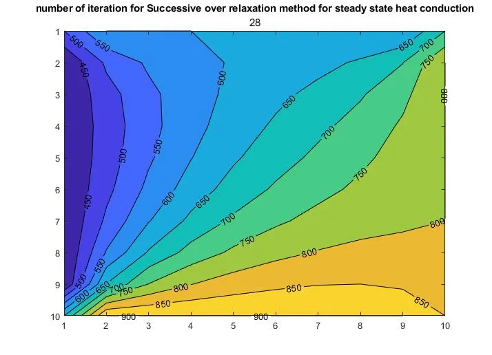
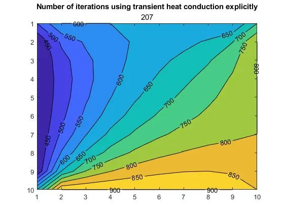
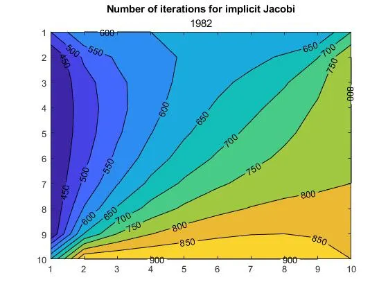
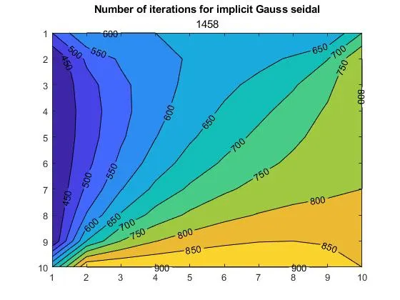
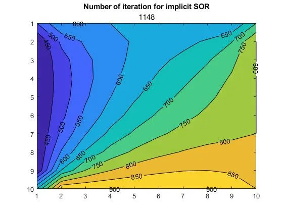
Conclusion:
The implicit method can be used for solving the problems when the converged results are needed in less computation time when they are unconditionally stable and the convergence rate will increase with the time step size which leads to a steady state with less number of iterations.