Week 5.1 - Mid term project - Solving the steady and unsteady 2D heat conduction problem
%function for steady state heat conction

function T=jocobi_method_solver(dx,dy,k,T,Told,nx,ny,tol,error,jocobi_iter,x,y)

while (error>tol)
for i=2:nx-1
    for j=2:ny-1

    term1=((Told(i-1,j)+Told(i+1,j)))/(k*dx^2);
    term2=((Told(i,j-1)+Told(i,j+1)))/(k*dy^2);
    T(i,j)=term1+term2;
end
error=max(max(abs(T-Told)));
Told=T;
jocobi_iter=jocobi_iter+1;


figure(1)
clabel(contourf(x,y,T))
%clabel(x,y,T) labels only the contour levels specified by vector T.
    colorbar
%     colorbar Display color bar (color scale)
    colormap(jet)
%      colormap is a function that sets the Colormap property of a figure

    xlabel('X-Axis')
    ylabel('Y-Axis')
    title(sprintf('No. of steady jocobian Iterations = %d', jocobi_iter));

end
end
%function for steady state heat condyction
function T=jocobi_method_solver(dx,dy,k,T,Told,nx,ny,tol,error,jocobi_iter,x,y)
while (error>tol)
for i=2:nx-1
for j=2:ny-1
term1=((Told(i-1,j)+Told(i+1,j)))/(k*dx^2);
term2=((Told(i,j-1)+Told(i,j+1)))/(k*dy^2);
T(i,j)=term1+term2;
end
error=max(max(abs(T-Told)));
Told=T;
jocobi_iter=jocobi_iter+1;
figure(1)
clabel(contourf(x,y,T))
%clabel(x,y,T) labels only the contour levels specified by vector T.
colorbar
% colorbar Display color bar (color scale)
colormap(jet)
% colormap is a function that sets the Colormap property of a figure
xlabel('X-Axis')
ylabel('Y-Axis')
title(sprintf('No. of steady jocobian Iterations = %d', jocobi_iter));
end
end%fuction for steady state heat conction using sor method
function T=sor_method(dx,dy,k,T,Told,nx,ny,tol,error,sor_iter,x,y,alpha)
while (error>tol)
for i=2:nx-1
for j=2:ny-1
term1=((Told(i-1,j)+Told(i+1,j)))/(k*dx^2);
term2=((Told(i,j-1)+Told(i,j+1)))/(k*dy^2);
T(i,j)=Told(i,j)*(1-alpha)+(alpha*(term1+term2));
end
error=max(max(abs(T-Told)));
Told=T;
sor_iter=sor_iter+1;
figure(1)
clabel(contourf(x,y,T))
%clabel(x,y,T) labels only the contour levels specified by vector T.
colorbar
% colorbar Display color bar (color scale)
colormap(jet)
% colormap is a function that sets the Colormap property of a figure
xlabel('X-Axis')
ylabel('Y-Axis')
title(sprintf('No. of steady jocobian Iterations = %d', sor_iter));
end
end%function for unsteady heat conction using jocobal solver
function T=jocobi_method_solver_unsteady(dx,dy,k,T,Told,nx,ny,tol,error,jocobi_iter,x,y,k1,k2)
while (error>tol)
for i=2:nx-1
for j=2:ny-1
term1=1/(1+2*k1+2*k2);
term2=k1*term1;
term3=k2*term1;
H=(Told(i-1,j))+(Told(i+1,j));
V=(Told(i,j-1)+Told(i,j+1));
T(i,j)=(Told(i,j)*term1)+(H*term2)+(V*term3);
end
error=max(max(abs(T-Told)));
Told=T;
jocobi_iter=jocobi_iter+1;
figure(2)
clabel(contourf(x,y,T))
%clabel(x,y,T) labels only the contour levels specified by vector T.
colorbar
% colorbar Display color bar (color scale)
colormap(jet)
% colormap is a function that sets the Colormap property of a figure
xlabel('X-Axis')
ylabel('Y-Axis')
title(sprintf('No. of unsteady jocobian Iterations = %d', jocobi_iter));
pause(0.003)
end
end%function for unsteady state heat conduction using guass seildle method
function T=gs_method_solver_unsteady(dx,dy,k,T,Told,nx,ny,tol,error,gs_iter,x,y,k1,k2)
while (error>tol)
for i=2:nx-1
for j=2:ny-1
term1=1/(1+2*k1+2*k2);
term2=k1*term1;
term3=k2*term1;
H=(T(i-1,j))+(Told(i+1,j));
V=(T(i,j-1)+Told(i,j+1));
T(i,j)=(Told(i,j)*term1)+(H*term2)+(V*term3);
end
error=max(max(abs(T-Told)));
Told=T;
gs_iter=gs_iter+1;
figure(2)
clabel(contourf(x,y,T))
%clabel(x,y,T) labels only the contour levels specified by vector T.
colorbar
% colorbar Display color bar (color scale)
colormap(jet)
% colormap is a function that sets the Colormap property of a figure
xlabel('X-Axis')
ylabel('Y-Axis')
title(sprintf('No. of unsteady gauss seidel Iterations = %d', gs_iter));
pause(0.003)
end
end%function for steady state heat conduction usiong sor method
function T=sor_method_solver_unsteady(dx,dy,k,T,Told,nx,ny,tol,error,sor_iter,x,y,k1,k2,alpha1)
while (error>tol)
for i=2:nx-1
for j=2:ny-1
term1=1/(1+2*k1+2*k2);
term2=k1*term1;
term3=k2*term1;
H=(Told(i-1,j))+(Told(i+1,j));
V=(Told(i,j-1)+Told(i,j+1));
Z=(Told(i,j)*term1)+(H*term2)+(V*term3);
T(i,j)=((Told(i,j)*(1-alpha1))+(alpha1*Z));
end
error=max(max(abs(T-Told)));
Told=T;
sor_iter=sor_iter+1;
figure(2)
clabel(contourf(x,y,T))
%clabel(x,y,T) labels only the contour levels specified by vector T.
colorbar
% colorbar Display color bar (color scale)
colormap(jet)
% colormap is a function that sets the Colormap property of a figure
xlabel('X-Axis')
ylabel('Y-Axis')
title(sprintf('No. of unsteady sor Iterations = %d', sor_iter));
pause(0.003)
end
end%main program
clear all
close all
clc
nx=10;
ny=nx;
dt=0.01;
alpha1=1.2;
alpha=2;
x=linspace(0,1,nx);
y=x;
dx=x(2)-x(1);
dy=dx;
[x y]=meshgrid(x,y);
T=ones(nx,ny);
T(1,:)=900;
T(end,:)=600;
T(:,1)=400;
T(:,end)=800;
k1=alpha*dt/dx^2;
k2=alpha*dt/dy^2;
Told=T;
tol=1e-4;
error=1;
k=(2*(dx^2+dy^2)/(dx^2*dy^2));
itteration_solver=input('enter itteration solver')
if itteration_solver==1
jocobi_iter=1;
tic
T=jocobi_method_solver(dx,dy,k,T,Told,nx,ny,tol,error,jocobi_iter,x,y);
T=jocobi_method_solver_unsteady(dx,dy,k,T,Told,nx,ny,tol,error,jocobi_iter,x,y,k1,k2);
jocobi_iter;
time=toc
end
if itteration_solver==2
tic
gs_iter=1
T=guass_seidel_method(dx,dy,k,T,Told,nx,ny,tol,error,gs_iter,x,y)
T=gs_method_solver_unsteady(dx,dy,k,T,Told,nx,ny,tol,error,gs_iter,x,y,k1,k2)
time=toc
end
if itteration_solver==3
sor_iter=1;
tic
T=sor_method(dx,dy,k,T,Told,nx,ny,tol,error,sor_iter,x,y,alpha1)
% T=sor_method_solver_unsteady(dx,dy,k,T,Told,nx,ny,tol,error,sor_iter,x,y,k1,k2,alpha1)
time=toc
end
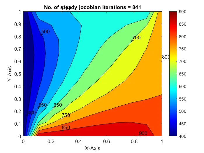
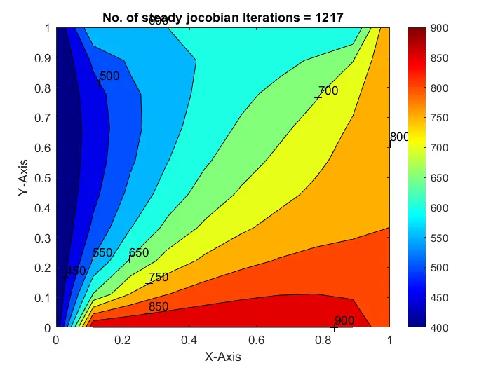
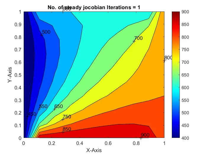
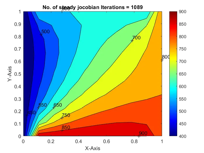
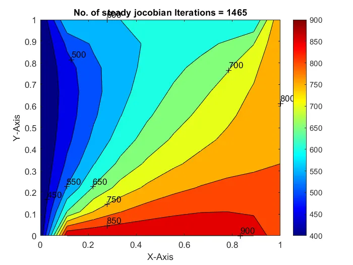
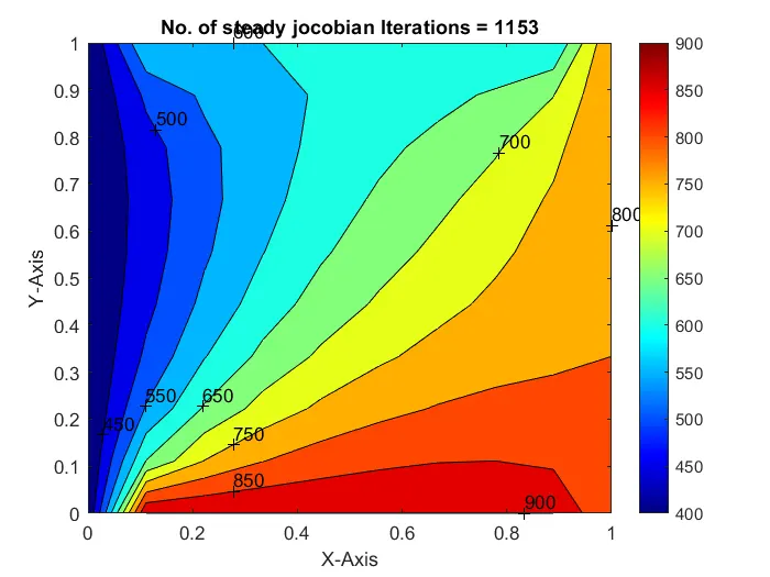
Aim:-Solve the 2D heat conduction equation by using the point iterative techniques using matlab
Governing eqn :-
for steady state heat conduction
`((d^2(T))/dx^2)+((d^2(T))/dy^2)=0`
for jocobi method
T(i,j)=((Told(i-1,j)+Told(i+1,j)))/(k*dx^2)+((Told(i,j-1)+Told(i,j+1)))/(k*dy^2)=Tj
for guass seidle method
T(i,j)=((T(i-1,j)+Told(i+1,j)))/(k*dx^2)+((T(i,j-1)+Told(i,j+1)))/(k*dy^2)=Tgs
for sor method
T(i,j)=Told(i,j)*(1-alpha1)+alpha1*(Tj or Tgs)
for unsteady state or transiaent state joconi method
term1=1/(1+2*k1+2*k2)
term2=k1*term1
term3=k2*term1
H=(Told(i-1,j))+(Told(i+1,j))
V=(Told(i,j-1)+Told(i,j+1))
T(i,j)=(Told(i,j)*term1)+(H*term2)+(V*term3)
here k1=alpha*dt/dx^2=k2
for unsteady stete using guass seidel method
term1=1/(1+2*k1+2*k2)
term2=k1*term1
term3=k2*term1
H=(Told(i-1,j))+(Told(i+1,j))
V=(Told(i,j-1)+Told(i,j+1))
T(i,j)=(Told(i,j)*term1)+(H*term2)+(V*term3)
here k1=alpha*dt/dx^2=k2
for unsteady stete using sor mrthod
term1=1/(1+2*k1+2*k2);
term2=k1*term1;
term3=k2*term1;
H=(Told(i-1,j))+(Told(i+1,j));
V=(Told(i,j-1)+Told(i,j+1));
Z=(Told(i,j)*term1)+(H*term2)+(V*term3);
T(i,j)=((Told(i,j)*(1-alpha1))+(alpha1*Z))
Body of content:-
intially the functions are defined using the governing eeqn
once the funtion is defined the in main prograam input alll the required input
then enter the solver which one want to be used to solve the pde
once the input and the requied paramets enter thime to run the program using the result the countour plot is ploted
Conclusion:-
for jocbian method the taken simulation time is more because it use the old value for one itteration hence the number of itterartion is also more compraed to th gs metyhod
for guass seidel method the time take is less compared to joccobian method here it so beuase in single ieteration the T takes updeted value from prvious step
for sor method its totally dependent on the alpha value if it is less than one and jocobian method is implimented it doeds thake more time if alpha is moer then the resulat may be obtained early or may not obtain ant result