Week 5.1 - Mid term project - Solving the steady and unsteady 2D heat conduction problem

Aim: Steady state analysis & Transient State Analysis

Conduction:

Conduction is the process by which heat energy is transmitted through collisions between neighboring atoms or molecules. Conduction occurs more readily in solids and liquids, where the particles are closer together than in gases, where particles are further apart. The rate of energy transfer by conduction is higher when there is a large temperature difference between the substances that are in contact.

The main difference between steady state and unsteady state/Transient heat transfer is that in steady-state the temperature at a point in the object does not change with respect to time while in the case of the unsteady state heat transfer the temperature at a specific point in the object increases or decreases with respect to time.

Steady state:

• The steady state heat transfer is denoted by, (∂t/∂τ = 0).
• The temperature of the object doesn’t vary with respect to time
• No heat diffusion occurs in the object.
• For the steady-state heat transfer, the energy entering the object is equal to the energy leaving from the object, Ein = Eout.
•     The change in the internal energy of the object is zero.

Unsteady state:

• The unsteady state heat transfer is denoted by, (∂t/∂τ ≠ 0).
• The temperature of the object changes with respect to time.
• Heat diffusion occurs in the object.
• For the unsteady state heat transfer, the energy entering the object is not equal to the energy leaving from the object, Ein ≠ Eout.
• The change in the internal energy of the object is not equal to zero.

 % conduction of 2D plate
clc
clear all
close all

n_x=6;
n_y=6;
L_x=1;
L_y=1;

dx = L_x/n_x;
dy = L_y/n_y;


% x = linspace(0,Lx,nx);
% y = linspace(0,Ly,ny);
% 
% T = meshgrid(x,y)

T=300*ones(n_x,n_y);  % array of temp

%BC
TL=400;
TR=800;
TT=600;
TB=900;

T(:,1)=TL;
T(:,end)=TR;
T(1,:)=TT;
T(end,:)=TB;

T(1,1)=0.5*(TL+TT);
T(1,end)=0.5*(TR+TT);
T(end,1)= 0.5*(TL+TB);
T(end,end)=0.5*(TR+TB);

%copy
T_old=T;
T_initial=T;

tol = 1e-4;
error = 1;


%Jacobian solver
jacob_iter=1;
while(error>tol)

    for j=2:n_y-1
        for i=2:n_x-1
          TL = T_old(i,j-1); TR = T_old(i,j+1); TT = T_old(i-1,j); TB = T_old(i+1,j);
          T(i,j) = 0.25*(TL + TR + TT + TB );
        end
    end

jacob_iter = jacob_iter+1;
error = max(max(abs(T-T_old)));
T_old = T;

figure(1)
contourf(flipud(T),'ShowText','on')
title_text=sprintf('Jacobian teration number=%d',jacob_iter)
title(title_text)
colorbar

end
   
% Re-initialize fields
T_gs = T_initial;
T_old = T_initial;


% Gauss-Seidel solver
iter_gs = 1;
error_gs =1;
while(error_gs>tol)

for j = 2:n_y-1
    for i = 2:n_x-1
    TL = T_gs(i,j-1); TR = T_gs(i,j+1); TT = T_gs(i-1,j); TB = T_gs(i+1,j);
    T_gs(i,j) = 0.25*(TL + TR + TT + TB );     
    end
end

iter_gs = iter_gs+1;
error_gs = max(max(abs(T_gs-T_old)));
T_old = T_gs;

figure(2)
contourf(flipud(T_gs),'ShowText','on')
title_text=sprintf('GS teration number=%d',iter_gs);
title(title_text)
colorbar

end

% Re-initialize fields
T_gs = T_initial;
T_SOR = T_initial;
T_old = T_initial;

%
iter_SOR = 1;
error_SOR = 1;

r = 1.5;
while(error_SOR>tol)

for j = 2:n_y-1
    for i = 2:n_x-1
    TL = T_gs(i,j-1); TR = T_gs(i,j+1); TT = T_gs(i-1,j); TB = T_gs(i+1,j);
    T_gs(i,j) = 0.25*(TL + TR + TT + TB ); 
    T_SOR(i,j) = (1-r)*T_old(i,j) + r*T_gs(i,j);
    end
end

iter_SOR = iter_SOR+1;
error_SOR = max(max(abs(T_SOR-T_old)));
T_old = T_SOR;

figure(3)
contourf(flipud(T_SOR),'ShowText','on')
title_text=sprintf('SOR Iteration number=%d',iter_SOR);
title(title_text)
colorbar
end

% 2D HEAT CONDUCTION ON A FLAT PLATE - TRANSIENT STATE
clear all
close all
clc
%Given_formulae:
%T(i,j)=T_prev(i,j)*(1-2k1-2k2)+K1(TR+TL)+k2(TT+TB)

%  EXPLICIT METHOD


n_x = 6;
n_y = 6;
L_x = 1;
L_y = 1;

d_x = L_x/n_x;
d_y = L_y/n_y;

% x = linspace(0,Lx,nx);
% y = linspace(0,Ly,ny);
% 
% T = meshgrid(x,y)

T = 300*ones(n_x,n_y);

TL = 400;
TR = 800;
TT = 600;
TB = 900;

T(:,1) = TL;
T(:,end) = TR;
T(1,:) = TT;
T(end,:) = TB;

T(1,1) = 0.5*(TL+TT);
T(1,n_x) = 0.5*(TR+TT);
T(n_y,1) = 0.5*(TL+TB);
T(n_x,n_y) = 0.5*(TR+TB);

%CFL

%K1=alpha*dt/dx^2
%k2=alpha*dt/dy^2
alpha=0.1;
d_t=1e-2;

K1=alpha*d_t/(d_x)^2;
K2=alpha*d_t/(d_y)^2;

%copy__
T_prev=T;
T_initial=T;

error=1;
tol=1e-4;

iter=1;

n_t=100 ;   
 %Time Convergence__Loop
 for k=1:n_t
  while(error>tol)
      
      %Space_Loop

       for j=2:n_y-1
        for i=2:n_x-1
            TL = T_prev(i,j-1); TR = T_prev(i,j+1); TT = T_prev(i-1,j); TB = T_prev(i+1,j);
            H=(TL+TR);V=(TT+TB);
            PR=(1-2*K1-2*K2);
            T(i,j) = T_prev(i,j)*PR + H*K1 + V*K2;
         end
       end
      iter=iter+1;
      error = max(max(abs(T-T_prev)));
      T_prev=T;

  
  end
 end
figure(1)
contourf(flipud(T),'ShowText','on')
title_text=sprintf('Explicit Iteration=%d',iter);
title(title_text)
colorbar

% 2D HEAT CONDUCTION ON A FLAT PLATE - TRANSIENT STATE
clear all
close all
clc
%Given_formulae:
%T(i,j)=T_old(i,j)+K1(TR+TL)+k2(TT+TB)/(1+2k1+2k2)

% IMplicit METHOD


n_x = 10;
n_y = 10;
L_x = 1;
L_y = 1;

d_x = L_x/n_x;
d_y = L_y/n_y;

% x = linspace(0,Lx,nx);
% y = linspace(0,Ly,ny);
% 
% T = meshgrid(x,y)
% Current time level matrix
T = 300*ones(n_x,n_y);
TL = 400;
TR = 800;
TT = 600;
TB = 900;

T(:,1) = TL;
T(:,end) = TR;
T(1,:) = TT;
T(end,:) = TB;

T(1,1) = 0.5*(TL+TT);
T(1,n_x) = 0.5*(TR+TT);
T(n_y,1) = 0.5*(TL+TB);
T(n_x,n_y) = 0.5*(TR+TB);


% CFL 
d_t =1e-2;
alpha = 0.3;
k1 = alpha*d_t/d_x^2;
k2 = alpha*d_t/d_y^2;
CFL = k1+k2;

tol = 1e-4;
error = 1;

% Copy__
T_prev = T;
T_old=T;
T_initial=T;
n_t=100;

iter=1;
for K=1:n_t
  error = 1; 
    %Convergence_Loop
    while(error>tol)
       %Space__Loop
        for j=2:n_y-1
            for i=2:n_x-1
               TL = T_old(i,j-1); TR = T_old(i,j+1); TT = T_old(i-1,j); TB = T_old(i+1,j);
                H=(TL+TR);V=(TT+TB);
                PR=1+2*k1+2*k2;
                T(i,j)= (T_prev(i,j) +H*k1 +V*k2)/(PR);
            end
        end    
        
       iter=iter+1;
       error = max(max(abs(T-T_old)));
       T_old=T;

    end
   T_prev=T;
end
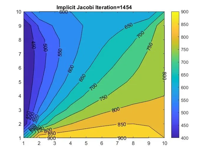
figure(1)
contourf(flipud(T),'ShowText','on')
title_text=sprintf('Implicit Jacobi Iteration=%d',iter);
title(title_text)
colorbar

% Re-initialize fields
T_gs = T_initial;
T_old = T_initial;
T_prev = T_initial;

iter_gs=1;
for K=1:n_t
  error = 1; 
    %Convergence_Loop
    while(error>tol)
       %Space__Loop
        for j=2:n_y-1
            for i=2:n_x-1
               TL = T_gs(i,j-1); TR = T_gs(i,j+1); TT = T_gs(i-1,j); TB = T_gs(i+1,j);
                H=(TL+TR);V=(TT+TB);
                PR=1+2*k1+2*k2;
               T_gs(i,j)= (T_prev(i,j) +H*k1 +V*k2)/(PR);
            end
        end    
        
       iter_gs=iter_gs+1;
       error = max(max(abs(T_gs-T_old)));
       T_old=T_gs;

    end
   T_prev=T_gs;
end
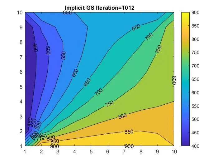
figure(2)
contourf(flipud(T_gs),'ShowText','on')
title_text=sprintf('Implicit GS Iteration=%d',iter_gs);
title(title_text)
colorbar

% Re-initialize fields
T_sor = T_initial;
T_old = T_initial;
T_prev = T_initial;

iter_sor=1;
r = 1.2;
for K=1:n_t
  error = 1; 
    %Convergence_Loop
    while(error>tol)
       %Space__Loop
        for j=2:n_y-1
            for i=2:n_x-1
               TL = T_sor(i,j-1); TR = T_sor(i,j+1); TT = T_sor(i-1,j); TB = T_sor(i+1,j);
                H=(TL+TR);V=(TT+TB);
                PR=1+2*k1+2*k2;
               T_GS(i,j)= (T_prev(i,j) +H*k1 +V*k2)/(PR);
               T_sor(i,j) = (1-r)*T_old(i,j) + r*T_GS(i,j);
            end
        end    
        
       iter_sor=iter_sor+1;
       error = max(max(abs(T_sor-T_old)));
       T_old=T_sor;

    end
   T_prev=T_sor;
end
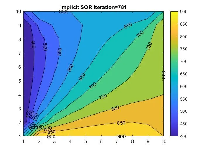
figure(3)
contourf(flipud(T_sor),'ShowText','on')
title_text=sprintf('Implicit SOR Iteration=%d',iter_sor);
title(title_text)
colorbar

Code explanation:

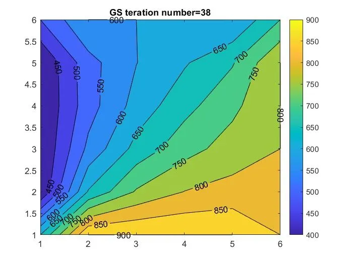
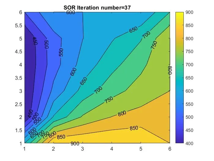
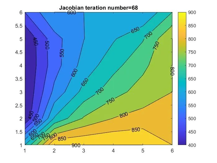
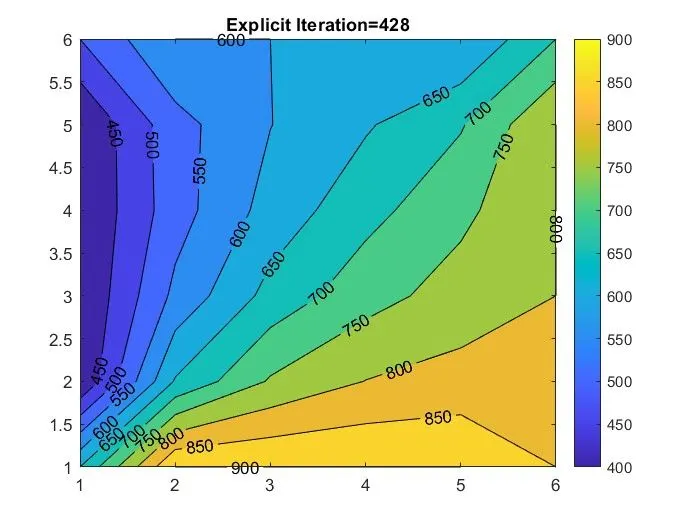
First to be remember that heat transfer due to temp differnence ie., the transfer takes place  from higher temp to lower temp b/w them at any point ,untill its attains  themal equillibrium at a point ,the state of equilibrium is nothing but no heat transfer because  the objects ie.,no temp diff b/w them . The above graphs clearly explains that the transfer/diffuses from higher temp to Low temp here the simulation explains that.Here the steady_state solvers & Transient solvers related to molecular structure of system °ree of molecular activity can be viewed as k.E& P.E energies of molecules ,its sum is called as Internal Energies of a system.The portion of internal energy of a system associated with the avg velocities of molecules or kinetic energies of molecules proportional to temp of gas or liquids.

The above explanation can be  viewed by Simulation at a point by  collecting information from the neighbouring points/nodes If we provide a value at apoint and this value influence temp in all neighbouring points,In order to compute temp at apoint we have to use information from all neighbouring points.we need to provide boundary conditions in all boundaries because if the information is being affected by all directions then we need to provide boundary conditions for entire domain.its an Elliptic PDE.Ths solvers take different time approches and no of iterations to solve the PDEs,but results in the same. Tha main difference of Explicit & Implicit is that,in the Emplicit which it takes information from the  neighbouring points from previous time steps (n) where as in the Implicit it takes the information from the current time steps(n+1).This is above explanation which i can give .