Challenge

Week 5.1 - Mid term project - Solving the steady and unsteady 2D heat conduction problem

SSuruguri Vinay9 Jun 2022

AIM : The main aim of the challange is to solve steady and unsteady state 2D heat conduction equation by using the iterative techniques such as Jaobi method, Gauss-seidal method & Successive over-relaxation method for both implicit and expliit scheme using mathlab.

The assumption for solving the problem :

Assume that the domain is to be a square.
Assume nx = ny [Number of points along the x direction is equal to number of points of points along y direction].
We are assuming nx = ny as 10.
Boundary conditions for steady and unsteady/ transient case,

Left = 400, Right = 800, Top = 600 Bottom = 900.

5. A part from the boundary conditions, all other nodes are given an initial temperature of 300k.

6. We implement the following methods.

Jacobi method
Gauss-seidal method
Successive over relaxation method.

Theory :

Consider general three dimensional heat conduction equation which has both time derivative and the spatial terms.

`partialT/partialt + alpha(partial^2T/partialx^2 + partial^2T/partialy^2 + partial^2T/partialz^2) = 0`

The above equation has two terms where, term 1 represents time derivative and time 2 is spatial derivative and where alpha is thermal diffusivity.

Now by consideribg the assumptions that the above equation is solved for a thin plate, dimensions in the z direction are neglected, thereby the above equation is convertes into the following form which is as follows.

`partialT/partialt + alpha(partial^2T/partialx^2 + partial^2T/partialy^2) = 0`

The above equation can be calculated by considering two approaches :

1. Steady state equation :

Under these conditions, the rate of change of temperature remains 0. Therefore in this condition time, the derivative term is equated to zero.

Steady state 2D heat conduction equation :

`partial^2T/partialx^2 +partial^2T/partialy^2 = 0`.

2. Unsteady state equation :

Under these conditions, both terms are considered therefore the equation is follwes as :

`partialT/partialt + alpha(partial^2T/partialx^2 + partial^2T/partialy^2)`= 0

Above two equations can be solved in 2 ways by using 3 iterative methods such as jacobi, gauss-seidal and SOR.

Implicit method.
Explicit method.

Solving the steady-state equation :

Consider two dimensional state steady equation

`partial^2T/partialx^2 + partial^2T/partialy^2 = 0`

after discretising above equation :

`T(i,j) = 1/K{(Told(i-1,j)+Told(i+1,j)/dx^2) + (Told(i,j-1)+Told(i,j+1)/dy^2)}`

`K = 2*(dx^2+dy^2/dx^2*dy^2)`

JACOBI ITERATION [STEADY-STATE] :

CODE :

clear all
close all
clc

% Solving the steady state 2D heatconduction (Jacobi methdo)

% Input conditions 
% Number of nodes 
nx = 10;
ny = nx;

x = linspace(0,1,nx);
y = linspace(0,1,ny);

dx = x(2) - x(1);
dy = dx;

% Absolute error criteria>tolerance
error = 9e9;
tolerance = 1e-4;

% Input boundary conditions 
T_L = 400;
T_T = 600;
T_R = 800;
T_B = 900;

T = 300*ones(nx,ny);

T(2:ny-1,1) = T_L;
T(2:ny-1,nx) = T_R;
T(1,2:nx-1) = T_T;
T(ny,2:nx-1) = T_B;

% Calculating average temperature at corners
T(1,1) = (T_T + T_L)/2;
T(nx,ny) = (T_R +T_B)/2;
T(1,ny) = (T_T + T_R)/2;
T(nx,1) = (T_L + T_B)/2;
 
% Assigning original values of T
T_intial = T;
T_old = T;

% Calculating of 2D steady heat conduction equation by jacobi method
iterative_solver = 1;

if iterative_solver == 1
    jacobi_iteration = 1;
    while(error > tolerance)
        for i = 2:nx -1
            for j = 2:ny-1
                T(i,j) = 0.25*(T_old(i-1,j) + T_old(i+1,j) + T_old(i,j-1) + T_old(i,j+1));
            end
        end
        error = max(max(abs(T_old - T)));
        T_old = T;
        jacobi_iteration = jacobi_iteration + 1;
    end
end

% Plotting 
figure(1)
contourf(x,y,T)
clabel(contourf(x,y,T))
colorbar
colormap("jet")
set(gca,'ydir','reverse')

xlabel('x-axis')
ylabel('y-axis')
title(sprintf('No. of jacobi iterations(IMPLICIT) = %d', jacobi_iteration));
pause(0.03);

PLOT :

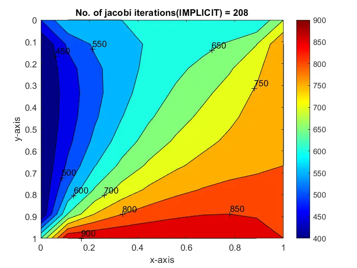
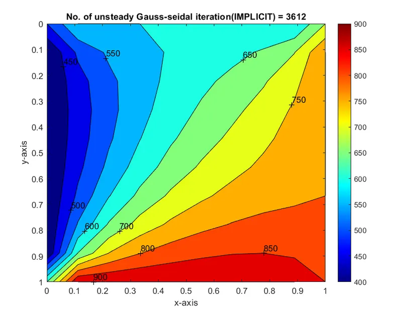
GAUSS SEIDAL ITERATION [STEADY-STATE] :

CODE :

clear all
close all
clc

% Solving the steady state 2D heat conduction (Gauss-seidel method)

% Input conditions 
% Number of nodes 
nx = 10;
ny = nx;

x = linspace(0,1,nx);
y = linspace(0,1,ny);

dx = x(2) - x(1);
dy = dx;

% Absolute error criteria>tolerance
error = 9e9;
tolerance = 1e-4;

% Defining boundary conditions 
T_L = 400;
T_T = 600;
T_R = 800;
T_B = 900;

T = 300*ones(nx,ny);

T(2:ny-1,1) = T_L;
T(2:ny-1,nx) = T_R;
T(1,2:nx-1) = T_T;
T(ny,2:nx-1) = T_B;

% Calculating average temperature at corners
T(1,1) = (T_T + T_L)/2;
T(nx,ny) = (T_R +T_B)/2;
T(1,ny) = (T_T + T_R)/2;
T(nx,1) = (T_L + T_B)/2;
 
% Assigning original values of T
T_intial = T;
T_old = T;

% Calculating of 2D steady heat conduction equation by gauss-seidel method
iterative_solver = 2;

if iterative_solver == 2
    Gauss_seidel_iteration = 1;
    while(error > tolerance)
        for i = 2:nx -1
            for j = 2:ny-1
                T(i,j) = 0.25*(T(i-1,j) + T_old(i+1,j) + T(i,j-1) + T_old(i,j+1));
            end
        end
        error = max(max(abs(T_old - T)));
        T_old = T;
        Gauss_seidel_iteration = Gauss_seidel_iteration + 1;
    end
end

% Plotting 
figure(1)
contourf(x,y,T)
clabel(contourf(x,y,T))
colorbar
colormap("jet")
set(gca,'ydir','reverse')

xlabel('x-axis')
ylabel('y-axis')
title(sprintf('No. of Gauss-seidel interations(IMPLICIT) = %d', Gauss_seidel_iteration));
pause(0.03);

PLOT :

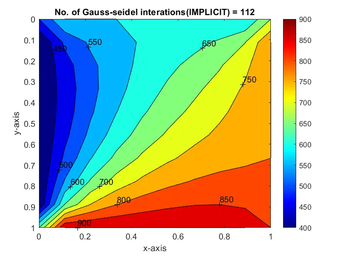
SUCCESSIVE OVER RELAXATION ITERATION [STEADY-STATE] :

CODE :

clear all
close all
clc

% Solving the steady state 2D heatconduction (Successive over-relaxation method)

% Input conditions 
% Number of nodes 
nx = 10;
ny = nx;

x = linspace(0,1,nx);
y = linspace(0,1,ny);

dx = x(2) - x(1);
dy = dx;

% Absolute error criteria>tolerance
error = 9e9;
tolerance = 1e-4;
omega = 1.2;

% Input boundary conditions 
T_L = 400;
T_T = 600;
T_R = 800;
T_B = 900;

T = 300*ones(nx,ny);

T(2:ny-1,1) = T_L;
T(2:ny-1,nx) = T_R;
T(1,2:nx-1) = T_T;
T(ny,2:nx-1) = T_B;

% Calculating average temperature at corners
T(1,1) = (T_T + T_L)/2;
T(nx,ny) = (T_R +T_B)/2;
T(1,ny) = (T_T + T_R)/2;
T(nx,1) = (T_L + T_B)/2;
 
% Assigning original values of T
T_intial = T;
T_old = T;

% Calculating of 2D steady heat conduction equation by Successive over-relaxation method
iterative_solver = 3;

if iterative_solver == 3
    successive_over_relaxation_iteration = 1;

    while(error > tolerance)
        for i = 2:nx -1
            for j = 2:ny-1
                T(i,j) = omega*(0.25*(T(i-1,j) + T_old(i+1,j) + T(i,j-1) + T_old(i,j+1))) + (1-omega)*T_old(i,j);
            end
        end
        error = max(max(abs(T_old - T)));
        T_old = T;
        successive_over_ralaxation_iteration = successive_over_relaxation_iteration + 1;
    end
end

% Plotting 
figure(1)
contourf(x,y,T)
clabel(contourf(x,y,T))
colorbar
colormap("jet")
set(gca,'ydir','reverse')

xlabel('x-axis')
ylabel('y-axis')
title(sprintf('No. of Successive over-ralaxation iterations(IMPLICIT)= %d', successive_over_relaxation_iteration));
pause(0.03);

PLOT :

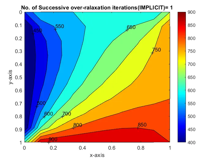
JACOBI ITERATION [UNSTEADY-STATE] :

CODE :

clear all
close all
clc

% Solving the unsteady state 2D heat conduction by jacobi method (IMPLICIT)

% Input parameters
% Number of grid points
nx = 10;
ny = nx;
nt = 1400;

x = linspace(0,1,nx);
y = linspace(0,1,ny);

dx = x(2)-x(1);
dy = dx;

% Absolute error criteria > tolerance
error = 9e9;
tolerance = 1e-4;
dt = 1e-3;

% Defining boundary conditions
T_L = 400;
T_T = 600;
T_R = 800;
T_B = 900;

T = 300*ones(nx,ny);

T(2:ny-1,1) = T_L;
T(2:ny-1,nx) = T_R;
T(1,2:nx-1) = T_T;
T(ny,2:nx-1) = T_B;

% Calculating average temperature at corners
T(1,1) = (T_T + T_L)/2;
T(nx,ny) = (T_R + T_B)/2;
T(1,ny) = (T_T + T_R)/2;
T(nx,1) = (T_L + T_B)/2;

% Assigning original values of T 
T_old = T;
T_initial = T;

% Calculation of 2D steady heat conditionequation by successive over relaxation method
k1 = 1.1*(dt/(dx^2));
k2 = 1.1*(dt/(dy^2));

jacobi_iteration = 1;
for k = 1:nt
    error = 9e9;
    while(error>tolerance)
        for i = 2:nx-1
            for j = 2:ny-1
                Term_1 = 1/(1+(2*k1)+(2*k2));
                Term_2 = k1*Term_1;
                Term_3 = k2*Term_1;
                H = (T_old(i-1,j)) + (T_old(1+i,j));
                V = (T_old(i,j+1)) + (T_old(i,j-1));

                T(i,j) = (T_initial(i,j)*Term_1)+(H*Term_2)+(V*Term_3);
            end
        end

        error = max(max(abs(T_old-T)));
        T_old = T;
        jacobi_iteration = jacobi_iteration+1;
    end

    T_initial = T;

    % Plotting 
    figure(1)
    contourf(x,y,T)
    clabel(contourf(x,y,T))
    colorbar
    colormap("jet")
    set(gca,'ydir','reverse')

    xlabel('x-axis')
    ylabel('y-axis')
    title(sprintf('No. of unsteady jacobi iterations(EXPLICIT) = %d', jacobi_iteration));
    pause(0.03)
end

PLOT :

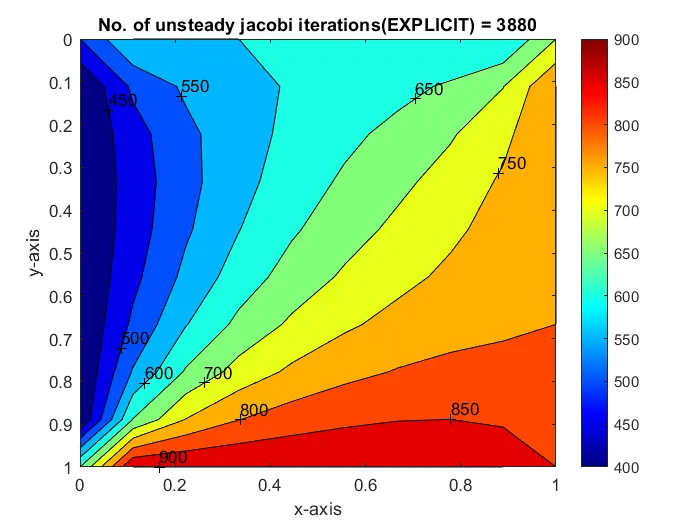
GAUSS SEIDEL ITERATION [UNSTEADY-STATE] :

CODE :

clear all
close all
clc

% Solving the unsteady state 2D heat conduction by Gauss seidel method (IMPLICIT)

% Input parameters
% Number of grid lines 
nx = 10;
ny = nx;
nt = 1400;

x = linspace(0,1,nx);
y = linspace(0,1,ny);

dx = x(2)-x(1);
dy = dx;

% Absolute error criteria > tolerance
error = 9e9;
tolerance = 1e-4;
dt = 1e-3;

% Defining boundary conditions
T_L = 400;
T_T = 600;
T_R = 800;
T_B = 900;

T = 300*ones(nx,ny);

T(2:ny-1,1) = T_L;
T(2:ny-1,nx) = T_R;
T(1,2:nx-1) = T_T;
T(ny,2:nx-1) = T_B;

% Calculating average temperature at corners
T(1,1) = (T_T + T_L)/2;
T(nx,ny) = (T_R + T_B)/2;
T(1,ny) = (T_T + T_R)/2;
T(nx,1) = (T_L + T_B)/2;

% Assigning original values to T
T_old = T;
T_initial = T;

% Calculation of 2D steady heat conduction equation by successive over relaxation method
k1 = 1.1*(dt/(dx^2));
k2 = 1.1*(dt/(dy^2));

gauss_seidel_iteration = 1;
for k = 1:nt
    error = 9e9;
    while(error>tolerance)
        for i = 2:nx-1
            for j = 2:ny-1
                Term_1 = 1/(1+(2*k1)+(2*k2));
                Term_2 = k1*Term_1;
                Term_3 = k2*Term_1;
                H = (T(i-1,j)) + (T_old(1+i,j));
                V = (T(i,j+1)) + (T_old(i,j-1));

                T(i,j) = (T_initial(i,j)*Term_1)+(H*Term_2)+(V*Term_3);
            end
        end

        error = max(max(abs(T_old-T)));
        T_old = T;
        gauss_seidel_iteration= gauss_seidel_iteration + 1;
    end

    T_initial = T;

    % Plotting 
    figure(1)
    contourf(x,y,T)
    clabel(contourf(x,y,T))
    colorbar
    colormap("jet")
    set(gca,'ydir','reverse')

    xlabel('x-axis')
    ylabel('y-axis')
    title(sprintf('No. of unsteady Gauss-seidal iteration(IMPLICIT) = %d', gauss_seidel_iteration));
    pause(0.03)
end

PLOT :

SUCCESSIVE OVER RELAXATION ITERATION [ UNSTEADY-STATE] :

CODE :

clear all
close all
clc

% Solving the unsteady state 2D heat conduction by Gauss seidel method (IMPLICIT)

% Input parameters
% Number of grid lines 
nx = 10;
ny = nx;
nt = 1400;

x = linspace(0,1,nx);
y = linspace(0,1,ny);

dx = x(2)-x(1);
dy = dx;

% Absolute error criteria > tolerance
error = 9e9;
tolerance = 1e-4;
dt = 1e-3;
omega = 1.1;

% Defining boundary conditions
T_L = 400;
T_T = 600;
T_R = 800;
T_B = 900;

T = 300*ones(nx,ny);

T(2:ny-1,1) = T_L;
T(2:ny-1,nx) = T_R;
T(1,2:nx-1) = T_T;
T(ny,2:nx-1) = T_B;

% Calculating average temperature at corners
T(1,1) = (T_T + T_L)/2;
T(nx,ny) = (T_R + T_B)/2;
T(1,ny) = (T_T + T_R)/2;
T(nx,1) = (T_L + T_B)/2;

% Assigning original values to T
T_old = T;
T_initial = T;
T_end = T;

% Calculation of 2D steady heat conduction equation by successive over relaxation method
k1 = 1.1*(dt/(dx^2));
k2 = 1.1*(dt/(dy^2));

successive_over_relaxation_iteration = 1;
for k = 1:nt
    error = 9e9;
    while(error>tolerance)
        for i = 2:nx-1
            for j = 2:ny-1
                Term_1 = 1/(1+(2*k1)+(2*k2));
                Term_2 = k1*Term_1;
                Term_3 = k2*Term_1;
                H = (T(i-1,j)) + (T_old(1+i,j));
                V = (T(i,j+1)) + (T_old(i,j-1));

                T(i,j) = (T_initial(i,j)*Term_1)+(H*Term_2)+(V*Term_3);
                T_end(i,j) = ((1-omega)*T_old(i,j))+(T(i,j)*omega);
            end
        end

        error = max(max(abs(T_old-T)));
        T_old = T_end;
        successive_over_relaxation_iteration= successive_over_relaxation_iteration + 1;
    end

    T_initial = T_end;

    % Plotting 
    figure(1)
    contourf(x,y,T)
    clabel(contourf(x,y,T))
    colorbar
    colormap("jet")
    set(gca,'ydir','reverse')

    xlabel('x-axis')
    ylabel('y-axis')
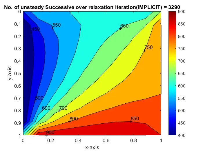
    title(sprintf('No. of unsteady Successive over relaxation iteration(IMPLICIT) = %d', successive_over_relaxation_iteration));
    pause(0.03)
end

PLOT :

EXPLICIT ITERATION :

CODE :

clear all
close all
clc
% Solving the unsteady state 2D heat conduction by (EXPLICIT)

% Input parameters
% Number of grid points
nx = 10;
ny = nx;
nt = 1400;

x = linspace(0,1,nx);
y = linspace(0,1,ny);

dx = x(2)-x(1);
dy = dx;

% Absolute error criteria > tolerance
error = 9e9;
tolerance = 1e-4;
dt = 1e-3;
omega = 1.1

% Defining boundary conditions
T_L = 400;
T_T = 600;
T_R = 800;
T_B = 900;

T = 300*ones(nx,ny);

T(2:ny-1,1) = T_L;
T(2:ny-1,nx) = T_R;
T(1,2:nx-1) = T_T;
T(ny,2:nx-1) = T_B;

% Calculating average temperature at corners
T(1,1) = (T_T + T_L)/2;
T(nx,ny) = (T_R + T_B)/2;
T(1,ny) = (T_T + T_R)/2;
T(nx,1) = (T_L + T_B)/2;

% Assigning original values of T 
T_old = T;
T_initial = T;

% Calculation of 2D steady heat conditionequation by successive over relaxation method
iterative_solver = 1;
k1 = 1.1*(dt/(dx^2));
k2 = 1.1*(dt/(dy^2));

if iterative_solver == 1;
    steady_explicit = 1;
    for k = 1:nt
        error = 1
    while(error > tolerance)
        for i = 2:nx-1
            for j = 2:ny-1
                Term_1 = T_old(i,j);
                Term_2 = k1*(T_old(i+1,j)-2*T_old(i,j)+(T_old(i-1,j)));
                Term_3 = k2*(T_old(i,j+1)-2*T_old(i,j)+T_old(i,j-1));
                T(i,j) = Term_1 + Term_2 + Term_3;
            end
        end

        error = max(max(abs(T_old-T)));
        T_old = T;
        steady_explicit  = steady_explicit+1;
    end
    end
end

    % Plotting 
    figure(1)
    contourf(x,y,T)
    clabel(contourf(x,y,T))
    colorbar
    colormap("jet")
    set(gca,'ydir','reverse')

    xlabel('x-axis')
    ylabel('y-axis')
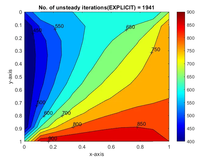
    title(sprintf('No. of unsteady iterations(EXPLICIT) = %d', steady_explicit));
    pause(0.03)

PLOT :

Conclusion :

1. In steady state equation SOR methods yields the results very quickly when compare to other two methids. Where as Jacobi method takes more time to solve the unknows. So the SOR method is most efficient when compared to other two methods to solve the steady state equation.

2. For transient equations, the time required to solve is more when compared to steady state equation. So, therefore it is recomended to solve the 2D heat conduction equation with steady state conditions.

In transient state equation, explicit methods yield the results quickly when compared to implicit method, but it is recomended under the solution when CFL is less than 0.25.

When transient state equation is solved implicitly SOR takes less time when compared to the other two methods where as gauss seidel is more stable when compared to Jacobi.

Week 5.1 - Mid term project - Solving the steady and unsteady 2D heat conduction problem

Ship work like this
in your own course.

Talk to a career counsellor

Ship work like thisin your own course.

Talk to a career counsellor

Ship work like this
in your own course.