Week 5.1 - Mid term project - Solving the steady and unsteady 2D heat conduction problem

The 2D Conduction two types are

1. Steady-state heat conduction
2. Un steady-state or transient heat conduction

`∂^2 T/ ∂x^2 + ∂^2 T / ∂y^2 + qg /k = 1/α * ∂T/∂t

T = Temperature

q = internal heat generation

α = Thermal diffusivity

Thermal diffusivity: It is defined as the ratio of the ability of medium conduct to heat to the ability of medium storage heat.

There is no internal heat generation and steady-state

steady-state heat transfer will not vary with respect to time

∂^2 T/ ∂x^2 + ∂^2 T = 0

unsteady-state: heat transfer varies with respect to time.

difference equation for steady and unsteady state

steady-state

T_p = 1/k [(T_R + T_L ) / Δx^2 + (T_T + T_B) / Δy^2

k = 2*[(Δx^2 + Δy^2 / Δx^2 *Δy^2)]

Transient heat conduction equation (explicit):

T_p ⁿ⁺¹ = T_p ⁿ + K1 [T_R ⁿ - 2 T_p ⁿ + T_L ⁿ ] + K2 [T_T ⁿ - 2 T_p ⁿ + T_B ⁿ ]

K1 = α (Δt / Δx^2)

K2 = α (Δt / Δy^2)

Implicit:

T_p ⁿ⁺¹ = 1/[1+2K1 + 2K2] + [T_P ⁿ + K1 ( T_R ⁿ+1 + T_L ⁿ⁺¹ ) + K2 [T_T ⁿ⁺¹ + T_B ⁿ⁺¹ ]

K1 = α (Δt / Δx^2)

K2 = α (Δt / Δy^2)

Main code:

clear all

close all

Clc

% Domain and discretization length

Number _node = 10;

domain_length = 1;

%value of x and y at nodes in a discretization plane

x = linspace(0,domain_length,number_node);

y = linspace(0,domain_length,number_node);

dx = domain_length (number _ node -1);

dy = domain_length( number_ node-1);

% Let define a temperature value at all nodes with initial guess 300k

T = 300 * ones(number _ node, number_ node);

% Initial boundary conditions at left and right

T(1:end,1) = 400;

T(1:end,end) = 800;

% Initial boundary conditions at bottom and top

T(end,1:end) = 900;

T(1,1: end) = 600;

% average values of T at corner boundaries:

T(1, 1 ) = 500;

T(end, 1 ) = 650;

T(1, end ) = 700;

T(end, end ) = 850;

%copy of Temperature to compute to compute

T_ old = T;

%constant

K = (2*(dx^2 + dy^2))/(dx^2*dy^2);

omegha = 1.2;

% to enter while loop initialize error value randomly

error = 10;

tol = 1e-4;

no _ iteration = 0;

method = input(‘enter(1) for jacobi,(2) for gauss siediel,(3) for sos’);

if method == 1

while(error>>tol)

for i = 2:number_node-1

for j . 2:numher_node-1

term 1 = (T _old(i+1,j )+T _ old(i-1,j))/ dx^2;

term 2 = (T _old(i,j+1 )+T _ old(i,j-1))/ dy^2;

T(i,j) = (term1 + term 2)/K;

end

end

error = max(max(abs(T_ old _ T)));

% to update the previous velocity with new velocity

%got from the iteration

T_ old = T;

no_iteration = no_iteration+1;

end

elseif method

while(error>to1)

for i = 2:number_node-1

for j = 2: number _ node-1

term 1 = (T _old(i+1,j )+T _ old(i-1,j))/ dx^2;

term 2 = (T _old(i,j+1 )+T _ old(i,j-1))/ dy^2;

T(i,j) = (term1 + term 2)/K;

end

error = max(max(abs(T_ old _ T)));

% to update the previous velocity with new velocity

% got from the iteration

T_ old = T;

no_iteration = no_iteration+1;

end

elseif method

while(error>to1)

for i = 2:number_node-1

for j = 2: number _ node-1

term 1 = (T _old(i+1,j )+T _ old(i-1,j))/ dx^2;

term 2 = (T _old(i,j+1 )+T _ old(i,j-1))/ dy^2;

T(i,j) = (1-omega)*T_ old(i,j)) + omega (term 1 + term 2 ) / k);

end

error = max(max(abs(T_ old _ T)));

% to update the previous velocity with new velocity

% got from the iteration

T_ old = T;

no_iteration = no_iteration+1;

end

end

% to visualize of result

[X, Y] = meshgrid(x,y);

Contour f(X,Y,T)

Color bar

Set (gca, ‘ ydir’, ‘reverse’,)

Unsteady state:

clear all

close all

Clc

% Domain and discretization length

Number _node = 10;

domain_length = 1;

%value of x and y at nodes in a discretization plane

x = linspace(0,domain_length,number_node);

y = linspace(0,domain_length,number_node);

dx = domain_length (number _ node -1);

dy = domain_length( number_ node-1);

% Let define a temperature value at all nodes with initial guess 300k

T = 300 * ones(number _ node, number_ node);

% Initial boundary conditions at left and right

T(1:end,1) = 400;

T(1:end,end) = 800;

% Initial boundary conditions at bottom and top

T(end,1:end) = 900;

T(1,1: end) = 600;

% average values of T at corner boundaries:

T(1, 1 ) = 500;

T(end, 1 ) = 650;

T(1, end ) = 700;

T(end, end ) = 850;

%copy of Temperature to compute to compute

T_ old = T;

% copy of T for previous time _ step

%constant

Alpha = 1.5 ;

omega = 1.15;

K 1 = (alpha * dt ) / dx^2;

K2 = (alpha *dt ) / dy^2;

Iteration = 0;

Approach = input( ‘Enter 1 for implicit or Enter 2 for explicit’)

if approach == 1

if method == 1

for nt = 1: 1500

error = 10;

to1 = 1e-4;

while(error>>to1)

for i = 2:number_node-1

for j = 2:numher_node-1

term 1 = 1 / 1+(2*k1) + (2*k2);

term 2 = k1* (T _ old(i+1, j) +T _ old(i-1,j));

term 3 = k2* (T _old (i, j+1 )+T _ old(i,j-1));

T(i,j) = term 1 *(T _ prev (i,j) + term 2 + term 3);

end

end

iteration = iteration + 1;

error = max(max(abs(T_ old _ T))));

T _ old = T;

End

T _ Prev = T;

End

elseif method == 2;

for nt = 1:1500

error = 10;

to1 = 1 e-4;

while (error>to1);

for i = 2:number_node-1

for j = 2: number _ node-1

term 1 = 1 / 1+(2*k1) + (2*k2);

term 2 = k1* (T _ old(i+1, j) +T _ old(i-1,j));

term 3 = k2* (T _old (i, j+1 )+T _ old(i,j-1));

T(i,j) = term 1 *(T _ prev (i,j) + term 2 + term 3);

end

end

iteration = iteration + 1;

error = max(max(abs(T_ old _ T))));

T _ old = T;

end

T _ Prev = T;

End

elseif method == 2;

for nt = 1:1500

error = 10;

to1 = 1 e-4;

while (error>to1);

for i = 2:number_node-1

for j = 2: number _ node-1

term 1 = 1 / 1+(2*k1) + (2*k2);

term 2 = k1* (T _ old(i+1, j) +T _ old(i-1,j));

term 3 = k2* (T _old (i, j+1 )+T _ old(i,j-1));

term 4 = term 1 *(T _ prev (i,j) + term 2 + term 3);

T(i,j) = ( 1 – omega) *(T _ old (i,j) + (omega * term 4);

end

end

iteration = iteration + 1;

error = max(max(abs(T_ old _ T))));

T _ old = T;

end

T _ Prev = T;

end

end

else

for nt = 1:1500

for i = 2:number_node-1

for j = 2:number_node-1

term 1 = k1* (T _ prev(i+1, j) - 2*T _ prev(i,j) + T _ Prev (i – 1 , j)));

term 2 = k2* (T _ prev(i,j+1) - 2*T _ prev(i,j) + T _ prev(i , j-1)));

T(i,j) = (T _ prev (i,j) + term 1 + term 2);

end

end

% to update the previous time step value with new time step value

% got from the iteration

T_ prev = T;

iteration = iteration+1;

end

end

% to visualize of result

[X, Y] = meshgrid(x,y);

Contour f(X,Y,T)

Color bar

Set (gca, ‘ ydir’, ‘reverse’,)

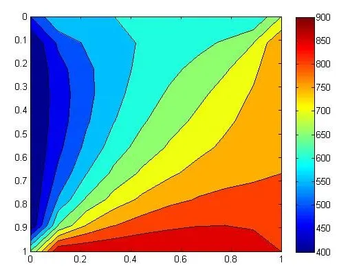
RESULT :

• The temperature distribution plot obtained for both the steady and unsteady conditions is the same.
• Because in Transient analysis also, the solution approaches to steady-state.
• The tap, bottom, left, and right side Of the graphs represent their respective boundary conditions.