Solving the steady and unsteady 2-D heat conduction equation using MATLAB
AIM: To solve the 2D heat conduction equation by using the point iterative techniques for steady-state and transient state analysis using Matlab.
GIVEN:
Top Boundary = 600 K
Bottom Boundary = 900 K
Left Boundary = 400 K
Right Boundary = 800 K
Absolute error criteria = 1e-4
OBJECTIVES:
- To solve the steady-state equation using the iterative solvers Jacobi method, Gauss-Seidel method, and the Successive Over Relaxation (SOR) method.
- To solve both implicitly and explicitly the transient/unsteady equation using the aforementioned solvers.
- To write the code and plot the results in Matlab and then compare the results.
THEORY:
Heat conduction can be defined as the transfer of thermal energy from the more energetic particles of a medium to the adjacent less energetic ones. It can take place in liquids and gases as well as solids if there is no bulk motion involved. The 3D transient heat conduction equation is given as-
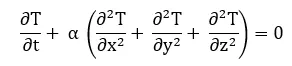
For this challenge, we shall be dealing with the 2D equation.
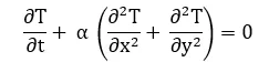
which can also be written as
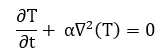
Steady-state and Transient (unsteady) state
Heat transfer problems are often classified as being steady (also called steady-state) or transient (also called unsteady). The term steady implies no change with time at any point within the medium, while transient implies variation with time or time dependence.
- Steady-state Analysis
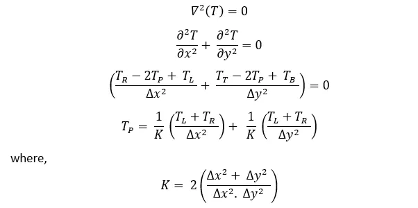
As explained above, for steady-state, the equation can now be written as-
- Transient or Unsteady-state Analysis
If we have a time-derivative term in the governing equation, as in this case, we use the time-marching solution. We discretize this using the Central-Difference Scheme for 2nd order terms (elliptical in nature, see figure below).
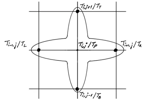

Here 'n' and 'n+1' are current and successive time-steps respectively. For simplification, we shall use the terms TP , TL , TR , TB, and TT. The equation can now be written as -

Simplifying, we get,
 (Explicit)
 (Implicit)
The implicit problems can be solved using the matrix method (difficult) or using the iterative solvers such as the Jacobi method, or Gauss-Seidel method, or the Successive Over Relaxation (SOR) method.
Now,
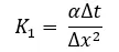

So, the final equation is -

CODE & RESULTS:
Assumptions-
- The domain is a unit square, L = 1
- An equal number of nodes in x and y, nx = ny
- error = 9e9
- Relaxataion factor, omega = 1.1
- Co-efficient of thermal diffusion, alpha = 1.4
1. Steady State
clear all
close all
clc

L = 1; %Length of the Domain
nx = 50; %Nodes
omega = 1.1;
error = 9e9;
tol = 1e-4;
ct = 0;
ny=nx;
x=linspace(0,L,nx);
dx=x(2)-x(1);
y=linspace(0,L,ny);
dy=y(2)-y(1);

T=300*ones(nx,ny);
T(:,1)= 400 ; %Left Wall
T(1,:)= 600; %Top Wall
T(:,end)= 800; %Right Wall
T(end,:)= 900; %Bottom Wall

T(1,1)= (400+600)/2 ;
T(1,end)= (600+800)/2 ;
T(end,1)= (400+900)/2 ;
T(end,end)= (900+800)/2 ;

Told = T;
k = 2*((dx^2+dy^2)/(dx^2*dy^2));

% Command prompt for choosing iterative solvers
prompt = 'Enter any one of the options and press Enter nChoose iterative solver type, 1 = Jacobi, 2 = Gauss-Seidel, 3 = SORn';
iterative_solver = input(prompt);

% method: 1.Jacobi 2. Gauss-Seidel , 3. SOR

if iterative_solver == 1
    tic
    Jacobi = 1;
    % Convergence Loop
    while(error>tol)
        % Space Loop
        for i = 2:nx-1
            for j = 2:ny-1
                H = ((Told(i-1,j)+ Told(i+1,j))/(k*dx^2));
                V = ((Told(i,j-1)+ Told(i,j+1))/(k*dy^2));
                T(i,j) = H+V;
            end
        end
        error = max(max(abs(Told - T)));
        Told = T;
        ct = ct + 1;

    end
    time = toc;
    figure(1)
    contourf(x,y,T,'ShowText','on');
    colorbar
    colormap(jet)
    xlabel('x');
    ylabel('y');
    text = sprintf('Steady State Heat Conduction n Method: Jacobi n No of iterations= %d n Time: %f s',ct ,time);
    title(text);
    set(gca,'YDIR','reverse');
end

if iterative_solver == 2
    tic
    Gauss_Seidel = 2;
    % Convergence Loop
    while(error>tol)
        % Space Loop
        for i = 2:nx-1
            for j = 2:ny-1
                H = ((T(i-1,j)+ Told(i+1,j))/(k*dx^2));
                V = ((T(i,j-1)+ Told(i,j+1))/(k*dy^2));
                T(i,j) = H+V;
            end
        end
        error = max(max(abs(Told - T)));
        Told = T;
        ct = ct + 1;
    end
    time = toc;
    figure(2)
    contourf(x,y,T,'ShowText','on');
    colorbar
    colormap(jet)
    xlabel('x');
    ylabel('y');
    text = sprintf('Steady State Heat Conduction n Method: Gauss-Seidel n No of iterations= %d n Time: %f s',ct ,time);
    title(text);
    set(gca,'YDIR','reverse');
end

if iterative_solver == 3
    tic
    SOR = 3;
    % Convergence Loop
    while(error>tol)
        % Space Loop
        for i = 2:nx-1
            for j = 2:ny-1
                H = ((T(i-1,j)+ Told(i+1,j))/(k*dx^2));
                V = ((T(i,j-1)+ Told(i,j+1))/(k*dy^2));
                T(i,j) = (1-omega)*(Told(i,j)) + (omega*(H + V));
            end
        end
        error = max(max(abs(Told - T)));
        Told = T;
        ct = ct + 1;

    end
    time = toc;
    figure(3)
    contourf(x,y,T,'ShowText','on');
    colorbar
    colormap(jet)
    xlabel('x');
    ylabel('y');
    text = sprintf('Steady State Heat Conduction n Method: SOR n No of iterations= %d n Time: %f s',ct ,time);
    title(text);
    set(gca,'YDIR','reverse');
end
OUTPUT:
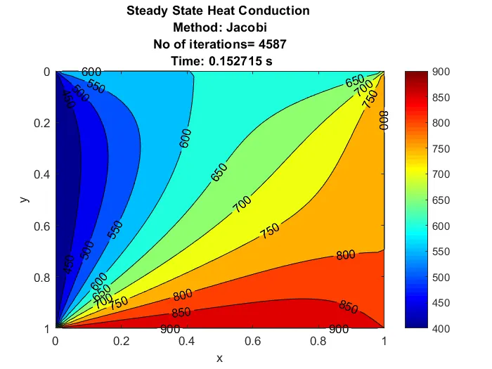
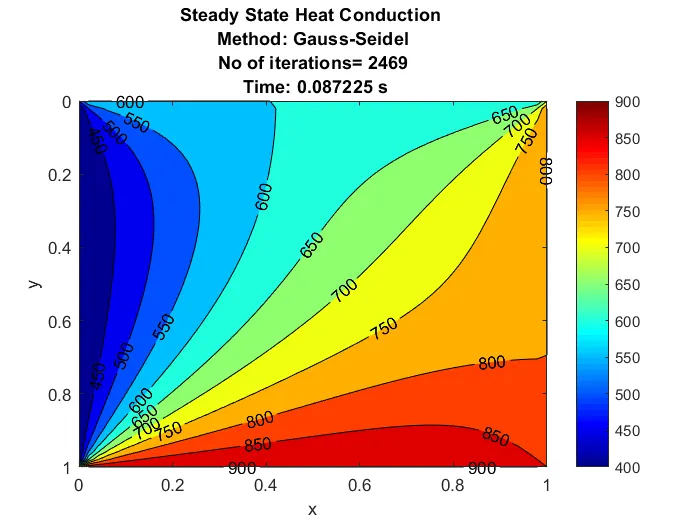
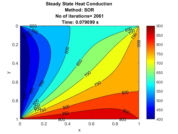
2. Unsteady-state (Explicit)
clear all
close all
clc

L = 1; %Length of the Domain
nx = 50; %Nodes
ny=nx;

x=linspace(0,L,nx);
dx=x(2)-x(1);
y=linspace(0,L,ny);
dy=y(2)-y(1);
t = 0.1;
nt = 1400;
dt = t/nt;
alpha = 1.4;
CFL_x= alpha*dt/(dx)^2;
CFL_y= alpha*dt/(dy)^2;
ct = 0;

T=300*ones(nx,ny);
T(:,1)= 400 ; %Left Wall
T(1,:)= 600; %Top Wall
T(:,end)= 800; %Right Wall
T(end,:)= 900; %Bottom Wall

T(1,1)= (400+600)/2 ;
T(1,end)= (600+800)/2 ;
T(end,1)= (400+900)/2 ;
T(end,end)= (900+800)/2 ;

Told = T;
k1 = (alpha*dt)/(dx^2);
k2 = (alpha*dt)/(dy^2);

tic
for k = 1:nt
    for i = 2:nx-1
        for j =2:ny-1
            H = (Told(i-1,j) - 2*Told(i,j) + Told(i+1,j));
            V = (Told(i,j+1) - 2*Told(i,j) + Told(i,j-1));
            T(i,j) = Told(i,j) + k1*H + k2*V;
        end
    end
    Told = T;
    ct = ct+1;
    time = toc;
end
figure(1)
contourf(x,y,T,'ShowText','on');
colorbar
colormap(jet)
xlabel('x');
ylabel('y');
text = sprintf(' Unsteady State Heat Conduction n Method: Explicit n No.of Iterations: %d n Time reqd.: %f',ct, time );
title(text);
set(gca,'YDIR','reverse');
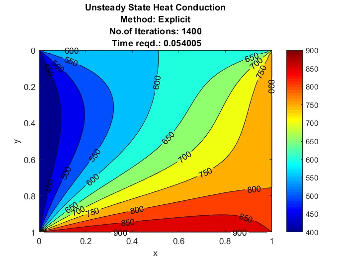
OUTPUT:
3. Unsteady-state (Implicit)
clear all
close all
clc

L = 1; %Length of the Domain
nx = 50; %Nodes
ny=nx;

x=linspace(0,L,nx);
dx=x(2)-x(1);
y=linspace(0,L,ny);
dy=y(2)-y(1);
t = 0.1;
nt = 1400;
dt = t/nt;
omega  = 1.1;
alpha = 1.4;
ct = 0;
error = 9e9;
tol = 1e-4;

T=300*ones(nx,ny);
T(:,1)= 400 ; %Left Wall
T(1,:)= 600; %Top Wall
T(:,end)= 800; %Right Wall
T(end,:)= 900; %Bottom Wall

T(1,1)= (400+600)/2 ;
T(1,end)= (600+800)/2 ;
T(end,1)= (400+900)/2 ;
T(end,end)= (900+800)/2 ;

Told = T;
T_prev = T;
k1 = (alpha*dt)/(dx^2);
k2 = (alpha*dt)/(dy^2);


prompt = 'Choose any one of the options and press Enter nChoose iterative solver type, 1 = Jacobi solver, 2 = GS Solver, 3 = SOR method n';
iterative_solver = input(prompt);

if iterative_solver == 1
    tic
    Jacobi = 1;
    for k = 1:nt
        error = 9e9;
        while(error>tol)
            for i = 2:nx-1
                for j =2:ny-1
                    term1 = 1/(1+2*k1+2*k2);
                    term2 = k1*term1;
                    term3 = k2*term1;
                    H = (Told(i-1,j) + Told(i+1,j));
                    V = (Told(i,j+1) + Told(i,j-1));
                    T(i,j) = (term1*(T_prev(i,j)))+(term2*H)+(term3*V);
                end
            end
            error = max(max(abs(Told-T)));
            Told = T;
            ct = ct+1;
        end
        T_prev = T;
    end
    time = toc;
    figure(1)
    contourf(x,y,T,'ShowText','on')
    colorbar
    colormap(jet)
    xlabel('X-axis');
    ylabel('Y-axis');
    text = sprintf('Unsteady State Heat ConductionnMethod: JacobinNo.of iterations: %dnTime: %f',ct, time);
    title(text);
    set(gca,'YDIR','reverse');
end

if iterative_solver == 2
    tic
    GS = 2;
    for k = 1:nt
        error = 9e9;
        while(error>tol)
            for i = 2:nx-1
                for j =2:ny-1
                    term1 = 1/(1+2*k1+2*k2);
                    term2 = k1*term1;
                    term3 = k2*term1;
                    H = (T(i-1,j) + Told(i+1,j));
                    V = (Told(i,j+1) + T(i,j-1));
                    T(i,j) = (term1*(T_prev(i,j)))+(term2*H)+(term3*V);
                end
            end
            error = max(max(abs(Told-T)));
            Told = T;
            ct = ct+1;
        end
        T_prev = T;
    end
    time = toc;
    figure(2)
    contourf(x,y,T,'ShowText','on')
    colorbar
    colormap(jet)
    xlabel('X-axis');
    ylabel('Y-axis');
    text = sprintf('Unsteady State Heat ConductionnMethod: Gauss-SeidelnNo.of iterations: %dnTime: %f',ct, time);
    title(text);
    set(gca,'YDIR','reverse');
end

if iterative_solver == 3
    tic
    SOR = 3;
    for k = 1:nt
        error = 9e9;
        while(error>tol)
            for i = 2:nx-1
                for j =2:ny-1
                    term1 = 1/(1+2*k1+2*k2);
                    term2 = k1*term1;
                    term3 = k2*term1;
                    H = (T(i-1,j) + Told(i+1,j));
                    V = (Told(i,j+1) + T(i,j-1));
                    T(i,j) = (1-omega)*(Told(i,j)) + (omega*((term1*(T_prev(i,j)))+(term2*H)+(term3*V)));
                end
            end
            error = max(max(abs(Told-T)));
            Told = T;
            ct = ct+1;
        end
        T_prev = T;
    end
    time = toc;
    figure(3)
    contourf(x,y,T,'ShowText','on')
    colorbar
    colormap(jet)
    xlabel('X-axis');
    ylabel('Y-axis');
    text = sprintf('Unsteady State Heat ConductionnMethod: SORnNo.of iterations: %dnTime: %f',ct, time);
    title(text);
    set(gca,'YDIR','reverse');
end
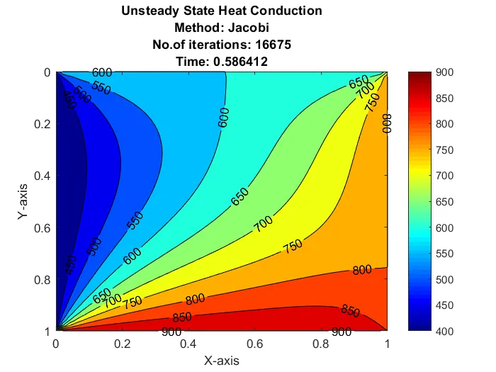
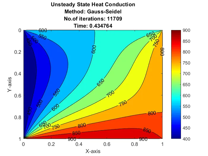
OUTPUT:
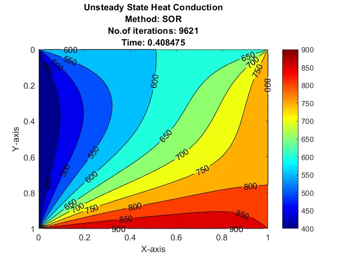
SUMMARY:
- To reach convergence, the number of iterations required for unsteady-state heat conduction analysis is more than the steady-state heat conduction analysis. Also, the number of iterations required for all the solvers in both the steady and unsteady cases to converge is as follows - Jacobi > Gauss-Seidel > SOR.
- Implicit solutions are unconditionally stable as the error is compared in each time-step.
- In Unsteady-state heat conduction analysis (explicit), no iterative solvers are required as all the terms on the RHS are known.
- The increase in the number of iterations required with the increase in the number of nodes used isn't linear, e.g. the number of iterations increases by a factor of approx. 4 when the number of nodes is increased by a factor of 2. This is a problem in large calculations and in those cases, faster solvers such as the conjugate gradient method, are used.
- Alpha can lead to faster convergence. However, if the alpha values are too high, it can also lead to divergence. Also, if omega >> 1, this results in overshooting and thereby can lead to oscillation.