Week 5.1 - Mid term project - Solving the steady and unsteady 2D heat conduction problem
AIM:
The objective of the report is to solve steady and unsteady state 2D heat conduction equation by using Implict and Explicit methods and validate the results.
PROCEDURE:
Given, Heat conduction equation
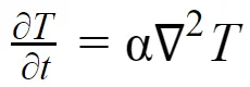
In 2D analysis, the above equation is written as
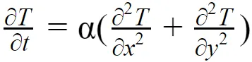
Where, T = Temperature
t = time
α = Thermal diffusivity
UNSTEADY STATE -
The unsteady/transient state equation is solved by using Implicit and Explicit methods.
1) EXPLICIT METHOD -
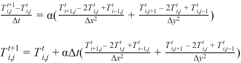
Explicit method is one of the numerical method for approximating the solution. In this method, the parameters of the current time step depends only on the previous time step parameters. For eg - T(n+1) = f(T(n)), here in this function temperature in n+1 time step depends on temperature in the nth time step.
The above equation is written as
2) IMPLICIT METHOD -
Implicit method is one of the numerical method for approximating the solution. In this method, the parameters of the current time step depends o the current as well as previous time step parameters. For eg - T(n+1) = f(T(n),T(n+1)), here in this function temperature in n+1 time step depend on n+1 , nth time step parameters.
The above equation is written as
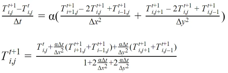
In Implicit method, by using some correction factor, the solution gets updated in each iteration until convergence is achieved.
In Implicit method, the equations are solved by using ITERATIVE solvers -
-
Jacobi - In this method, the node values at (i+1)th iteration is updated by using node values at (i)th iteration step.
- Gauss-seidel - In this method, the node values at (i+1)th iteration is updated by using (i)th and (i+1)th iteration step nodal values.
-
Successive over-relaxation - This method is a combination of Jacobi and Gauss-seidel method and relaxation factor is used to update the nodal values. For relaxation factor less than 1, takes more time to converge the solution than the relaxation factor greater than 1.
STEADY STATE -
In steady state equation, the time derivative term is zero. Since, no time derivative term present in the expression, there is no meaning of Implicit and Explicit methods in steady state analysis. So iterative solvers are used to compute the solution.
BOUNDARY CONDITIONS -
The domain of the problem is a unit square with equal number of grid points along x and y direction are considered. The following boundary conditions are given
T(left face) = 400K
T(rightface) = 800K
T(top face) = 600K
T(bottom face) = 900K
MATLAB CODE -
1) Transient state
clc;
clear all;
close all;

L = 1; %length of square domain
nx = 10;
ny = 10;
x = linspace(0,1,nx);
y = linspace(0,1,ny);
dx = L/nx;  %grid spacing along x-axis
dy = L/ny;  %grid spacing along y-axis

% initial value
T = 300*ones(10,10);

% boundary condition
T(:,1) = 400;  %left boundary
T(:,10) = 800;  %right boundary
T(1,:) = 600;  %top boundary
T(10,:) = 900;  %bottom boundary

Tinitial = T;
Told = T;
Tprev = T;
tol = 1e-4;   %tolerance limit value
error = 1;

alpha = 1.2;  %thermal iffusivity
dt = 0.002;   %time step
k1 = alpha*dt/dx^2;
k2 = alpha*dt/dy^2;

term1 = 1/(1+2*k1+2*k2);
term2 = k1*term1;
term3 = k2*term1;

iteration_value_jacobi = 0;
%Jacobi method
for nt = 1:500     %time loop
    error = 1;
    while(error > tol)  %convergence loop
        for j = 2:ny-1
            for i = 2:nx-1
                H = Told(i-1,j) + Told(i+1,j);
                V = Told(i,j-1) + Told(i,j+1);
                T(i,j) = term1*Tprev(i,j) + term2*H + term3*V;

            end
        end
        iteration_value_jacobi = iteration_value_jacobi + 1;
        error = max(max(abs(T - Told)));
        Told = T;
    end

    Tprev = T;
    figure(1)
    [c,h] = contourf(x,y,T);
    title('Jacobian method',['Total number of iterations =',num2str(iteration_value_jacobi)])
    xlabel('x-axis')
    ylabel('y-axis')
    clabel(c,h);
    colormap(jet)
    colorbar

end
Tjac_final_sol = T;


%gauss method
T = Tinitial;
Told = Tinitial;
Tprev = Tinitial;
tol = 1e-4;
error = 1;
iteration_value_gauss = 0;

for nt = 1:500     %time loop
    error = 1;
    while(error > tol)  %convergence loop
        for j = 2:ny-1
            for i = 2:nx-1
                H = T(i-1,j) + Told(i+1,j);
                V = T(i,j-1) + Told(i,j+1);
                T(i,j) = term1*Tprev(i,j) + term2*H + term3*V;

            end
        end
        error = max(max(abs(T - Told)));
        Told = T;
        iteration_value_gauss = iteration_value_gauss+1;
    end

    Tprev = T;
    figure(2)
    [c,h] = contourf(x,y,T);
    title('Gauss method',['Total number of iterations =',num2str(iteration_value_gauss)])
    xlabel('x-axis')
    ylabel('y-axis')
    clabel(c,h);
    colormap(jet)
    colorbar
end
Tgauss_final_sol = T;


%SOR method
T = Tinitial;
Told = Tinitial;
Tprev = Tinitial;
tol = 1e-4;
error = 1;
w = 1.2; %relaxation factor
iteration_value_sor = 0;

for nt = 1:500     %time loop
    error = 1;
    while(error > tol)  %convergence loop
        for j = 2:ny-1
            for i = 2:nx-1
                H = T(i-1,j) + Told(i+1,j);
                V = T(i,j-1) + Told(i,j+1);
                T(i,j) = (1-w)*Told(i,j) + w*(term1*Tprev(i,j) + term2*H + term3*V);

            end
        end
        iteration_value_sor = iteration_value_sor+1;
        error = max(max(abs(T - Told)));
        Told = T;
    end
    Tprev = T;
    figure(3)
    [c,h] = contourf(x,y,T);
    title('SOR method',['Total number of iterations =',num2str(iteration_value_sor)])
    xlabel('x-axis')
    ylabel('y-axis')
    clabel(c,h);
    colormap(jet)
    colorbar
end
Tsor_final_sol = T;


%%Explicit analysis
T = Tinitial;
Tprev = Tinitial;
tol = 1e-4;
steady_state_error = 1;
iteration_explicit = 0;

for nt = 1:500

    for j=2:ny-1
        for i = 2:nx-1
            H = Tprev(i-1,j) + Tprev(i+1,j);
            V = Tprev(i,j-1) + Tprev(i,j+1);
            T(i,j) = term1*Tprev(i,j) + term2*H + term3*V;
        end
    end

    iteration_explicit = iteration_explicit + 1;
    Tprev = T;

    figure(4)
    [c,h] = contourf(x,y,T);
    sc = num2str(iteration_explicit);
    title(['Explicit analysis'],['Iteration = ',sc])
    clabel(c,h);
    xlabel('x-axis')
    ylabel('y-axis')
    colormap(jet)
    colorbar
end
T_explicit_final_sol = T;
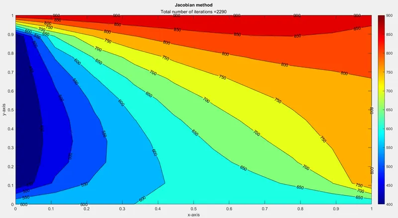
FIG 1 - IMPLICIT_JACOBIAN METHOD
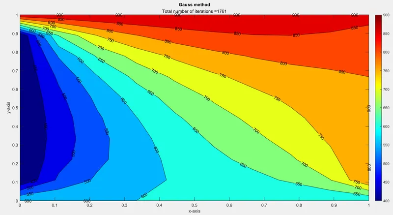
FIG 2 - IMPLICIT_GAUSS SEIDEL METHOD
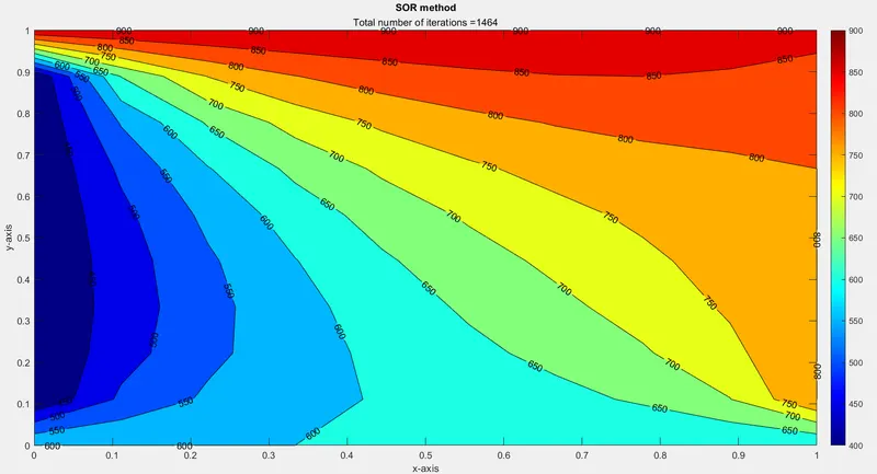
FIG 3 - IMPLICIT_SUCCESIVE OVER RELAXATION METHOD
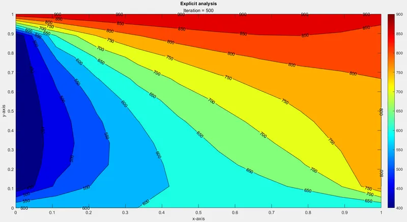
FIG 4 - EXPLICIT METHOD
The above fig shows the contour plots obtained by solving the transient state equation by using Implicit and Explicit methods. From fig 1,2,3,4 it is observed that the final solution obtained in all the methods are nearly same as the plots look similar. Out of all these methods, it is observed that Explicit method achieves convergence more quickly compared to Implicit method
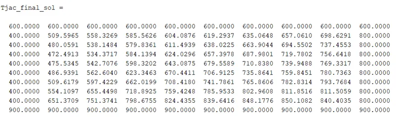
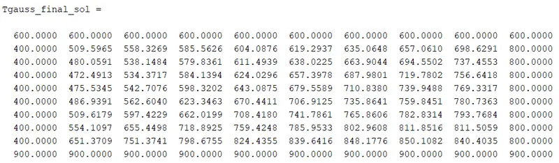
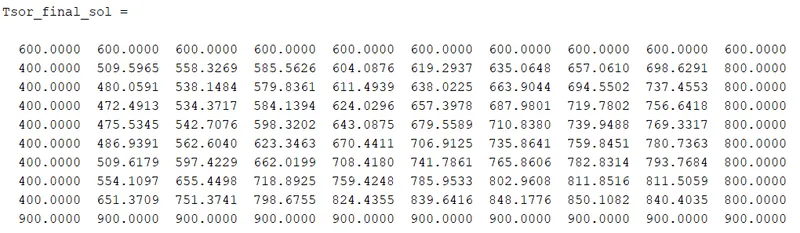
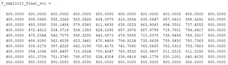
It is observed that the final obtained temperature values in the domain is same for all iterative solvers in Implicit method. For explicit method, when compared to Implicit method there is an error of order 1e-4 is observed. So, for Implicit methods better accurate solutions are achieved.
2) Steady state
clc;
clear all;
close all;
L = 1; %domain lenght along x&y axis
nx = 10; %10 nodes along x
ny = 10; %10 nodes along y
dx = L/nx;
dy = L/ny;
x = linspace(0,L,nx);
y = linspace(0,L,ny);

%initial guess values
T = 300*ones(nx,ny);

%boundary condition
T(:,1) = 400;  %left boundary
T(:,10) = 800;  %right boundary
T(1,:) = 600;  %top boundary
T(10,:) = 900;  %bottom boundary

Tinitial = T;
Told = T;

k1 = (dx^2*dy^2)/(2*dx^2*(dx^2+dy^2));
k2 = (dx^2*dy^2)/(2*dy^2*(dx^2+dy^2));

tol = 1e-4;
error = 1;
iter_value_jac = 0;
while(error > tol)
    iter_value_jac = iter_value_jac+1;
for j = 2:(ny-1)
    for i = 2:(nx-1)
        H = Told(i+1,j)+Told(i-1,j);
        V = Told(i,j+1)+Told(i,j-1);
        T(i,j) = k1*H + k2*V;
    end
end
error = max(max(abs(T - Told)));
Told = T;


figure(1)
[c,h] = contourf(x,y,T);
clabel(c,h);
colormap(jet)
colorbar
xlabel('x axis')
ylabel('y axis')
sc = num2str(iter_value_jac);
title('Jacobian method',['iteration =',sc])

end
Tjac_final_sol = T;

%gaussidian method
T = Tinitial;
Told = Tinitial;
error = 1;
iter_value_gauss = 0;

while(error > tol)
    iter_value_gauss = iter_value_gauss+1;
for j = 2:(ny-1)
    for i = 2:(nx-1)
        H = Told(i+1,j)+T(i-1,j);
        V = Told(i,j+1)+T(i,j-1);
        T(i,j) = k1*H + k2*V;

    end
end
error = max(max(abs(T - Told)));
Told = T;

figure(2)
[c,h] = contourf(x,y,T);
clabel(c,h);
colormap(jet)
colorbar
xlabel('x axis')
ylabel('y axis')
sc = num2str(iter_value_gauss);
title('Gauss method',['iteration =',sc])

end
Tgauss_final_sol = T;


%SOR method
w = 1.2;
T = Tinitial;
Told = Tinitial;
error = 1;
iter_value_sor = 0;

while(error > tol)
    iter_value_sor = iter_value_sor+1;
for j = 2:(ny-1)
    for i = 2:(nx-1)
       H = Told(i+1,j)+T(i-1,j);
       V = Told(i,j+1)+T(i,j-1);
       T(i,j) = (1-w)*Told(i,j) + w*(k1*H + k2*V);
    end
end
error = max(max(abs(T-Told)));
Told = T;


figure(3)
[c,h] = contourf(x,y,T);
clabel(c,h);
colormap(jet)
colorbar
xlabel('x axis')
ylabel('y axis')
sc = num2str(iter_value_sor);
title('SOR method',['iteration =',sc])

end
Tsor_final_sol = T;
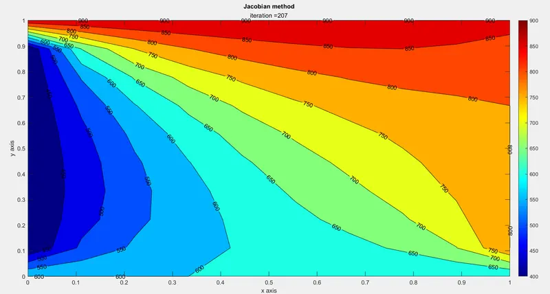
FIG 5 - EXPLICIT_JACOBIAN METHOD
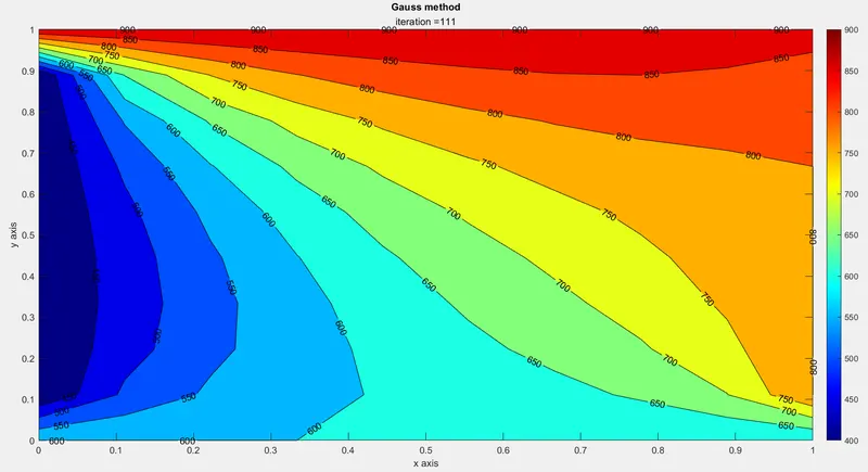
FIG 6 - EXPLICIT_GAUSS-SEIDEL METHOD
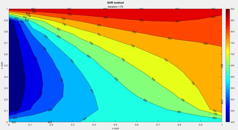
FIG 7 - EXPLICIT_SUCCESIVE OVER RELAXATION METHOD
The above fig shows the contour plots obtained by solving the steady state equation by using Implicit method. From fig 5,6,7 it is observed that the final solution obtained in all the methods are nearly same as the plots look similar. Out of all these methods, it is observed that successive over relaxation method achieves convergence more quickly compared to other iterative solvers.
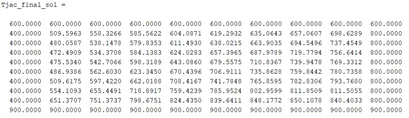
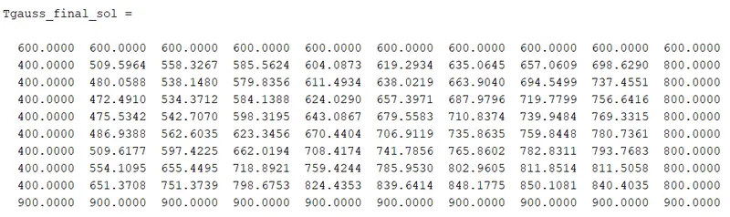
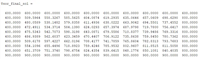
It is observed that the final obtained temperature values of steady state in the domain is same for all iterative solvers but an error of order of 1e-4 is observed. So, for Implicit methods better accurate solutions are achieved.