Developing numerical solver using iterative methods for Solving the steady and unsteady 2D heat conduction problem
AIM-To study behaviour of parabolic and elliptic differential equation (2-D heat conduction) unsteady/ steady through programming using point intervive techniques.
1. Given problem
2D Heat conduction (Transient and steady)
2. Boundary conditions
Top Boundary = 600 K
Bottom Boundary = 900 K
Left Boundary = 400 K
Right Boundary = 800 K
Absolute error criteria = 1e-4
Theory.
Part-I
Steady state:
Boundary conditions-
Top Boundary = 600 K
Bottom Boundary = 900 K
Left Boundary = 400 K
Right Boundary = 800 K
Absolute error criteria = 1e-4
The governing PDE for steady state heat conduction can be written as
`(del^2T)/(delx^2)+(del^2T)/(dely^2 ) = S_u(x,y)`
where solution `S_u`source term.
When source tends to zero poision equation is said to be laplace equation.
`(del^2T)/(delx^2)+(del^2T)/(dely^2 ) = 0`---------(1)
The above equation is elliptic in nature and the physical behaviour reflect by those equation will be equilibrium problems. An important feature of this kind of problem is
1. Any disturbance in the interior of the solution affects and alters the solution everywhere else
2. Disturbance signals travel in all direction through the interior solution. The solution of these kind problem are smooth even if the boundary conditions are discontinuous.
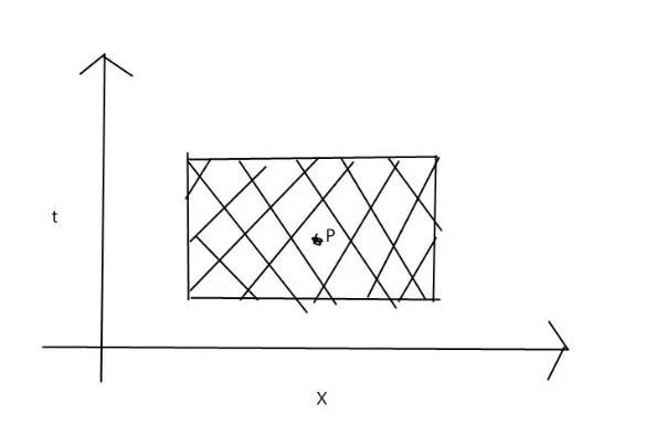
3. Boundary condition to be specified along the entire domain boundary, either in Dirichlet or Neuman from.
The equation (1) can be expanded in taylor series and doing some algebric manupulation, It can be expressed as:-
`(T_(i+1,j)^(n)-2T_(i,j)^n+T_(i-1,j)^(n))/(Deltax^2)+(T_(i,j+1)^(n)-2T_(i,j)^n+T_(i,j-1)^(n))/(Deltay^2)=0`----------(2)
Doing some algebric manupulation---- 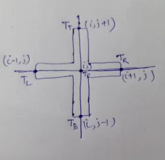
`T_p = 1/k(((T_l+T_k)/(Deltax^2))+((T_T+T_B)/(Deltay^2)))`-------(3)
`"Where" K = 2((Deltax^2+Deltay^2)/(Deltax^2Deltay^2))`
Equation (3) can be solved either by taking temperature from previous time step or can be solved at simultaneous time step. If It’s solving by taking temperature from previous time step it’s said to be explicit method else simultaneous way of solving system of equation is said to be implicit methods. Writing a program using explicit method is pretty straight forward but brings some condition for stable solution. Where as in implicit method programming is difficult but it’s unconditionally stable. Since it’s taking all the information at same time step and solving simultaneously ( It can also be proved using Von- neuman stability analysis ). Since in implicit method bunch of equation has to be solved simultaneously , So we need some iterative methods. Such as jacobi, Gauss seidel, successive over relaxation, Block iterative methods, chebyshev Iterative method, ADI, conjugate gradient method etc. from challenge point of view we will develop 3 iteravive methods such as Jacobi, Gauss seides and SOR and we will compare rate of convergence among them.
The solution is said to be converged when----
Two successive iteration levels locally at each grid point convergence has been achived i.e
(1) `abs(T_(i,j)^(k+1)-T_(i,j)^(k)`<= `epsilon` (where `epsilon` = Absolute error criteria)
Root mean squre iteration error
(2) `sqrt(sum(T_(i,j)^(k+1)-T_(i,j)^(k))^2/N`<=`epsilon`
where N= No of interior point
Iterative Methods
Point Jacobi
`T_(i,j)^(k+1) = 1/4[T_(i+1,j)^(k)+T_(i-1,j)^(k)+T_(i,j+1)^(k)+T_(i,j-1)^(k)]`
where `Deltax=Deltay = Delta`
Point Gauss-Seidel
`T_(i,j)^(k+1) = 1/4[T_(i+1,j)^(k)+T_(i-1,j)^(k+1)+T_(i,j+1)^(k)+T_(i,j-1)^(k+1)]`
where `Deltax=Deltay = Delta`
SOR
`T_(i,j)^(k+1) = T_(i,j)^(k) (1-alpha)+alpha(T_(jac))`
`T_(i,j)^(k+1) = T_(i,j)^(k) (1-alpha)+alpha(T_(gs))`
when `alpha <1`----- Under relaxation
`alpha= 1`-----Gauss seidel
`alpha>1`----- Over relaxation
N.B- 1. Numerical experiment are required to obtaion optimum value of `alpha` for a given problem
2. Over relaxation used for accelerated convergence
Matlab Code(Implicit)
% 2D Laplace equation
% 2-D heat Conduction problem
%steady
%d^2(T)/dx^2+d^2(T)/dy^2
%Solving Implicitely
%Jacobi
%Guss-seidel
%SOR


% discretization
% no of nodes
close all
clear all
clc

n = 11;
m = 11;
x = 0: 1/(n-1): 1;
y = 0: 1/(m-1): 1;
dx = x(2)-x(1);
dy = y(2)-y(1);
% step size
h = 1/(n-1);
k = 1/(m-1);


%co-efficient of Thermal conductivity
%unit = wt/m^2k

alpha = 1.5;
nt = 5000;


k_1 = .25;

[Y, X] = meshgrid(y,x);

% source = 0

% Initialising solution
T = ones(n);
%Dirichlet Boundary condition
T( :,1) = 400;
T( :,n) = 800;
T(1,: ) = 600;
T(n,: ) = 900;
T(1,1)    = 500;
T(1,n)  = 700;
T(n,1)  = 650;
T(end)  = 850;
T(2:n-1,2:n-1) = 300;
T_old = T;
% T_old = T;
% T_prev_gs = T;
T_prev_sor = T;
residual = 1e-5;
err = 10;

iterative_solver = 3;

tic

     jacobi_iter = 1;
     gs_iter = 1;
     sor_iter = 1;
   if iterative_solver == 1;


        err = 10;

        while (err>residual)
            T_old = T;
            for i = 2:n-1
                for j = 2:m-1
                    T(i,j) = .25*(T_old(i,j-1)+T_old(i,j+1)+T_old(i-1,j)+T_old(i+1,j));
                end
            end
            % Residual calcuation
            err = max(max(abs(T-T_old)));
            % Updating new Temperature profile
            T_old = T;
           jacobi_iter = jacobi_iter+1;

        end


        figure(1)
        colormap(jet)
        contourf(x,fliplr(y),T,'ShowText','on')

        xlabel('X axis')
        ylabel('Y')
        title_text = sprintf('iteration number = %d', jacobi_iter);
        title(title_text)
        colorbar
        end
% % guss-seidel
err = 10;
conv = 10;
t_iter = 0;
if iterative_solver == 2;
%Time loop

       T_old = T;
        err = 10;
        while (err>residual)
            for i = 2:n-1
                for j = 2:m-1
                    T(i,j)=.25*(T(i,j-1)+T_old(i,j+1)+T(i-1,j)+T_old(i+1,j));
                end
            end
            % Residual calcuation
            err = max(max(abs(T-T_old)));
            % Updating new Temperature profile
            T_old = T;
        gs_iter = gs_iter+1;
        Simulation_time_1 = toc;


        end


        figure(2)
        colormap(jet)
        contourf(x,fliplr(y),T,'ShowText','on')
        colorbar
        xlabel('X axis')
        ylabel('Y')
        title_text = sprintf('iteration number = %d', gs_iter);
        title(title_text)

        end


% Successive over relaxation

err = 10;
conv = 10;
t_iter = 0;
if iterative_solver == 3
    sor = 1.5;    %Relaxaation factor
    % sor = 1  GAUSS SEIDEL
    %sor = 0   JACOBI
    %sor < 1 under relaxation
    %sor > 1 over relaxation


%Time loop

       T_prev_sor = T;
        err = 10;
        while (err>residual)
            for i = 2:n-1
                for j = 2:m-1
                    T_GS =.25*(T(i,j-1)+T_old(i,j+1)+T(i-1,j)+T_old(i+1,j));
                    T(i,j) = (1-sor)*T_old(i,j) + sor*T_GS; %T_old in the place of T_prev_sor
                end
            end

            % Residual calcuation
            err = max(max(abs(T-T_old)));
            % Updating new Temperature profile
            T_old = T;
        sor_iter = sor_iter+1;
        Simulation_time_1 = toc;

        end

end

        figure(3)
        colormap(jet)
        contourf(x,fliplr(y),T,'ShowText','on')
        colorbar
        xlabel('X axis')
        ylabel('Y')
        title_text = sprintf('iteration number = %d', sor_iter);
        title(title_text)
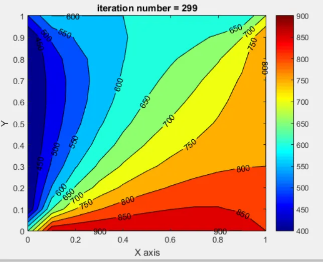
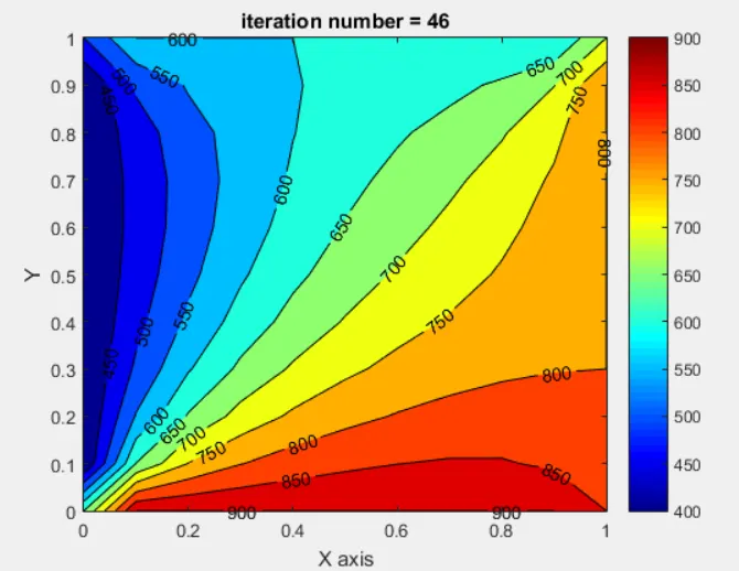
PLOT
JACOBI
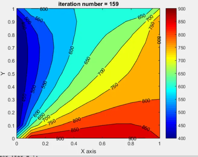
Gauss Seidel
SOR
MATLAB CODE (Explicit)
% 2D Laplace equation
% 2-D heat Conduction problem
%unsteady transient
%dT/dt+d^2(T)/dx^2+d^2(T)/dy^2
%Solving explicitely
% discretization
% no of nodes
close all
clear all
clc

n = 11;
m = 11;
x = 0: 1/(n-1): 1;
y = 0: 1/(m-1): 1;
dx = x(2)-x(1);
dy = y(2)-y(1);
% step size
h = 1/(n-1);
k = 1/(m-1);
%time step

nt =5000;
dt = .001;

%co-efficient of Thermal conductivity
%unit = wt/m^2k

alpha = 1.5;

% CFL Number

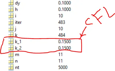
k_1 = (alpha*dt)/(dx)^2;
k_2 = (alpha*dt)/(dy)^2;


[Y, X] = meshgrid(y,x);

% source = 0

% Initialising solution
T = ones(n);
%Dirichlet Boundary condition
T( :,1) = 400;
T( :,n) = 800;
T(1,: ) = 600;
T(n,: ) = 900;
T(1,1)    = 500;
T(1,n)  = 700;
T(n,1)  = 650;
T(end)  = 850;
T(2:n-1,2:n-1) = 300;
T_old = T;
residual = 1e-5;
conv = 10;


tic

     iter = 0;

       for k=1:nt

            for i = 2:n-1
                for j = 2:m-1
                    T(i,j) = 0.25*(T(i,j-1)+T(i,j+1)+T(i-1,j)+T(i+1,j));

                end
            end

   conv = max(max(abs(T-T_old)));
if(conv < residual)
    break
end

            % Updating new Temperature profile
            T_old = T;
           iter = iter+1;
            figure(1)
        colormap(jet)
    contourf(x,fliplr(y),T,'ShowText','on')
    pause(0.01)
        colorbar
        xlabel('X axis')
        ylabel('Y')
        title_text = sprintf('iteration number = %d', iter);
        title(title_text)

        end
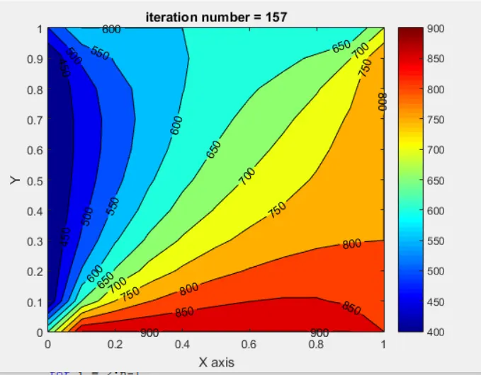
PLOT
The Governing PDE for unsteady heat conduction for 2-d can be writer as
`(delu)/(delt)=alpha((del^2t)/(delx^2)+(del^2t)/(dely^2))` -------------(1)
where `alpha`is thermal conductivity. (constant)
The above equation is parabolic PDE. As such it tends itself to a marching solution W.R.T time
The equation has 2 independent quantities x and t.
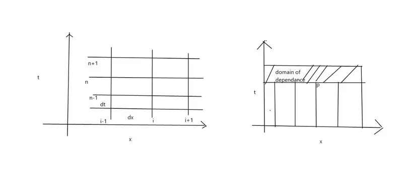
looking into above figure, i is the running index in x direction. ‘n’ is the running index in ‘t’ direction. Having said that the time derivative of above marching PDE can be written.
`((delu)/(delt))_(i,j)^n= (T_(i,j)^(n+1)-T_(i,j)^n)/(Deltat)-(del^2T)/(delt^2)((Deltat)/2)+....(FD Scheme)`------------(2`
and space term can be written as---
`((del^2T)/(delx^2))_(i,j)^n= (T_(i+1,j)^(n)-2T_(i,j)^n+T_(i-1,j)^(n))/(Deltax^2)-(del^4T)/(delx^4)((Deltax^2)/12)+..`----------(3`
Similarly observation can be extend to and derivatives.
`((del^2T)/(dely^2))_(i,j)^n= (T_(i,j+1)^(n)-2T_(i,j)^n+T_(i,j-1)^(n))/(Deltay^2)-(del^4T)/(dely^4)((Deltay^2)/12)+..`----------(4`
Combining equation 2,3,4
`(delu)/(delt)-alpha((del^2t)/(delx^2)+(del^2t)/(dely^2)) =0`
`(T_(i,j)^(n+1)-T_(i,j)^n)/(Deltat)-alpha((T_(i+1,j)^(n)-2T_(i,j)^n+T_(i-1,j)^(n))/(Deltax^2)+(T_(i,j+1)^(n)-2T_(i,j)^n+T_(i,j-1)^(n))/(Deltay^2))+[-(del^2T)/(delt^2)((Deltat)/2)+(alpha)(del^4T)/(delx^4)((Deltax^2)/12)+(alpha)(del^4T)/(dely^4)((Deltay^2)/12)]`-------(5)
`[-(del^2T)/(delt^2)((Deltat)/2)+(alpha)(del^4T)/(delx^4)((Deltax^2)/12)+(alpha)(del^4T)/(dely^4)((Deltay^2)/12)]` ------- Truncation error
Examining equation (5) left hand side is original PDE and right hand side is difference equation with trunction term. Also it is 1st order accurate in time and 2nd order accurate in space `O[Deltat,Deltax^2]`. Before going to solution method let’s have some observation from above difference equation…
From equation 5 The physical property (i.e tempereture) can be evaluate at each grid point by two methods. Either assuming properties at 'n'th time step or at 'n+1'th time step. If calculation done by taking nth time step the methods is called explicit method. If the calculation done by taking 'n+1'th time step, the methods is called Implicit method. Both the method has some extend of merit and demerits.
lets discuss one by one ----
Explicit method.
When solving a parabolic PDE with an explicit technique we ask the question will the time stepping calculations converge to a steady state solution ?
Ans:- stability of the finite difference scheme needs to be investigated using von-neuman stability analysis.
From the analysis it can be seen for stable solution diffusion term should be less than .5.
Implicit method (laasonner method)
- From Von-neuman stability analysis it can be seen its unconditionally stable.
- TDMA based solution.
3. `O[Deltat, Deltax^2]`
- As it comes with system of equations, Iteravive solver such as point jacabi, point guss-seidel, line Guss- seidel, point SOR etc. based algorithms needed to solve (effectivenes of different iterative solver explained in conclusion part with plot.
Matlab code for 2d unsteady heat conduction
Boundary conditions-
Top Boundary = 600 K
Bottom Boundary = 900 K
Left Boundary = 400 K
Right Boundary = 800 K
Absolute error criteria = 1e-4
MATLAB code (EXplicit solver)
% 2D Laplace equation
% 2-D heat Conduction problem
%unsteady transient
%dT/dt+d^2(T)/dx^2+d^2(T)/dy^2
%Solving explicitely
% discretization
% no of nodes
close all
clear all
clc

n = 11;
m = 11;
x = 0: 1/(n-1): 1;
y = 0: 1/(m-1): 1;
dx = x(2)-x(1);
dy = y(2)-y(1);
% step size
h = 1/(n-1);
k = 1/(m-1);
%time step

nt =5000;
dt = .001;

%co-efficient of Thermal conductivity
%unit = wt/m^2k

alpha = 1.5;

% CFL Number

k_1 = (alpha*dt)/(dx)^2;
k_2 = (alpha*dt)/(dy)^2;


[Y, X] = meshgrid(y,x);

% source = 0

% Initialising solution
T = ones(n);
%Dirichlet Boundary condition
T( :,1) = 400;
T( :,n) = 800;
T(1,: ) = 600;
T(n,: ) = 900;
T(1,1)    = 500;
T(1,n)  = 700;
T(n,1)  = 650;
T(end)  = 850;
T(2:n-1,2:n-1) = 300;
T_old = T;
residual = 1e-5;
conv = 10;


tic

     iter = 0;

       for k=1:nt

            for i = 2:n-1
                for j = 2:m-1
                    T(i,j) = T_old(i,j)+k_1*(T_old(i,j+1)-2*T_old(i,j)+T_old(i,j-1))...
                        +k_2*(T_old(i+1,j)-2*T_old(i,j)+T_old(i-1,j));
                end
            end

   conv = max(max(abs(T-T_old)));
if(conv < residual)
    break
end

            % Updating new Temperature profile
            T_old = T;
           iter = iter+1;
            figure(1)
        colormap(jet)
    contourf(x,fliplr(y),T,'ShowText','on')
    pause(0.01)
        colorbar
        xlabel('X axis')
        ylabel('Y')
        title_text = sprintf('iteration number = %d', iter);
        title(title_text)

        end
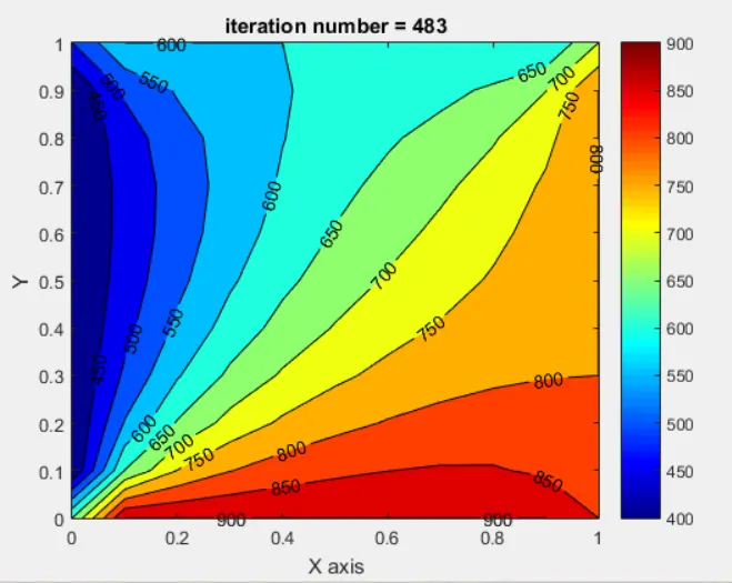
Plot
MATLAB code (Implicit solver)
For implicit method we will use iteretive solver such as-
1. Jacobi
The implementation of the Jacobi scheme follows the iterative formula

2. Gauss-Seidel Method
The implementation of the Gauss-Seidel Method follows the iterative formula

3. SOR Method
The implementation of the SOR follows the iterative formula
Jacobi-

Gauss-Seidel-

N.B-: Derivation to above formula will be discussed in Week-6 project in detailed manner. For this project reference has been taken from https://www.springer.com/gp/book/9789402412154
Chapter- 5
MATLAB code (Implicit solver)
% 2D Laplace equation
% 2-D heat Conduction problem
%unsteady transient
%dT/dt+d^2(T)/dx^2+d^2(T)/dy^2
%Solving Implicitely
%Jacobi
%Guss-seidel
%SOR


% discretization
% no of nodes
close all
clear all
clc

n = 11;
m = 11;
x = 0: 1/(n-1): 1;
y = 0: 1/(m-1): 1;
dx = x(2)-x(1);
dy = y(2)-y(1);
% step size
h = 1/(n-1);
k = 1/(m-1);
%time step


dt = 10;

%co-efficient of Thermal conductivity
%unit = wt/m^2k

alpha = 1.5;

% CFL Number

k_1 = (alpha*dt)/(dx)^2;
k_2 = (alpha*dt)/(dy)^2;
k_3 = (1+2*k_1+2*k_2)^-1*k_1;
k_4 = (1+2*k_1+2*k_2)^-1*k_2;

[Y, X] = meshgrid(y,x);

% source = 0

% Initialising solution
T = ones(n);
%Dirichlet Boundary condition
T( :,1) = 400;
T( :,n) = 800;
T(1,: ) = 600;
T(n,: ) = 900;
T(1,1)    = 500;
T(1,n)  = 700;
T(n,1)  = 650;
T(end)  = 850;
T(2:n-1,2:n-1) = 300;
T_old = T;
T_prev_j = T;
T_prev_gs = T;
T_prev_sor = T;
residual = 1e-4;
err = 10;
conv = 10;
iterative_solver = 3;

tic

     jacobi_iter = 1;
     gs_iter = 1;
     sor_iter = 1;
   if iterative_solver == 1;

       % Jacobi
%Time loop
while conv>residual

        err = 10;
        T_prev_j = T;
        while (err>residual)
            for i = 2:n-1
                for j = 2:m-1
                    T(i,j) = T_prev_j(i,j)*(1+2*k_1+2*k_2)^-1 +k_3*(T_old(i-1,j) ...
                        +T_old(i+1,j))+k_4*(T_old(i,j+1)+T_old(i,j-1));
                end
            end
            % Residual calcuation
            err = max(max(abs(T-T_old)));
            % Updating new Temperature profile
            T_old = T;
           jacobi_iter = jacobi_iter+1;

        end
     conv = max(max(abs(T-T_prev_j)));
end


        figure(1)
        colormap(jet)
        contourf(x,fliplr(y),T,'ShowText','on')

        xlabel('X axis')
        ylabel('Y')
        title_text = sprintf('iteration number = %d', jacobi_iter)
        title(title_text)
        colorbar
        end
% % guss-seidel
err = 10;
conv = 10;
t_iter = 0;
if iterative_solver == 2;
%Time loop
while conv>residual
       T_prev_gs = T;
        err = 10;
        while (err>residual)
            for i = 2:n-1
                for j = 2:m-1
                    T(i,j) = (T_prev_gs(i,j)+k_1*(T(i-1,j)+T_old(i+1,j))+k_2*(T_old(i,j+1)+T(i,j-1)))/(1+2*k_1+2*k_2);
                end
            end
            % Residual calcuation
            err = max(max(abs(T-T_old)));
            % Updating new Temperature profile
            T_old = T;
        gs_iter = gs_iter+1;
        Simulation_time_1 = toc;

        end
conv = max(max(abs(T-T_prev_gs)));
t_iter = t_iter+1;
end


        figure(2)
        colormap(jet)
        contourf(x,fliplr(y),T,'ShowText','on')
        colorbar
        xlabel('X axis')
        ylabel('Y')
        title_text = sprintf('iteration number = %d', gs_iter)
        title(title_text)

        end

% Successive over relaxation

err = 10;
conv = 10;
t_iter = 0;
if iterative_solver == 3
    sor = 1.5;    %Relaxaation factor
    % sor = 1  GAUSS SEIDEL
    %sor = 0   JACOBI
    %sor < 1 under relaxation
    %sor > 1 over relaxation


%Time loop
while conv>residual
       T_prev_sor = T;
        err = 10;
        while (err>residual)
            for i = 2:n-1
                for j = 2:m-1
                    T_GS = (T_prev_sor(i,j)+k_1*(T(i-1,j)+T_old(i+1,j))+k_2*(T_old(i,j+1)+T(i,j-1)))/(1+2*k_1+2*k_2);
                    T(i,j) = (1-sor)*T_old(i,j) + sor*T_GS; %T_old in the place of T_prev_sor
                end
            end

            % Residual calcuation
            err = max(max(abs(T-T_old)));
            % Updating new Temperature profile
            T_old = T;
        sor_iter = sor_iter+1;
        Simulation_time_1 = toc;

        end
conv = max(max(abs(T-T_prev_sor)));
t_iter = t_iter+1;
end

        figure(3)
        colormap(jet)
        contourf(x,fliplr(y),T,'ShowText','on')
        colorbar
        xlabel('X axis')
        ylabel('Y')
        title_text = sprintf('iteration number = %d', sor_iter)
        title(title_text)

 end
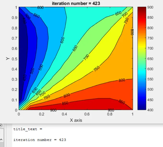
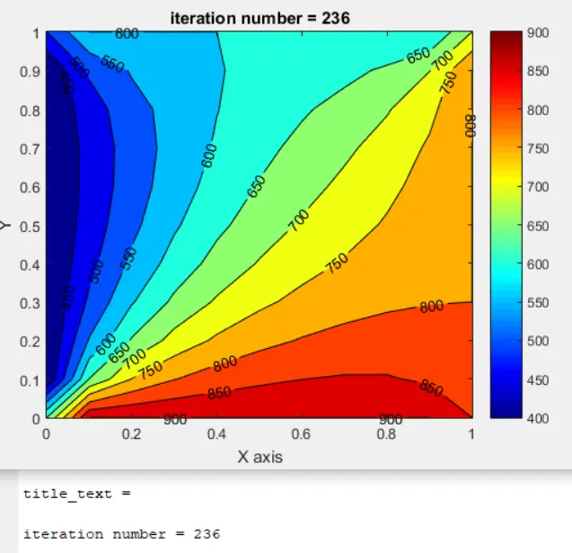
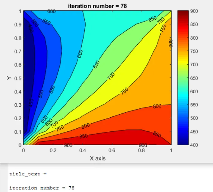
Plot
Jacobi
Gauss-Seidel
SOR
N.B-:
Implicit method- Solutions are unconditionally stable
Explicit method- Diffusion factor should be less than equal to .5 for stable solution.
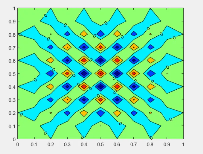
Unstable Solution
Diffusion Factor-1.5
Obsevation and Conclusion
EXPLICIT SCHEME CONVERGENCE RATE
| No of Iteration | ||
| Unsteady | 483 | |
| Steady | 157 |
IMPLICIT SCHEME CONVERGENCE RATE
| No of Iteration in Jacobi | No of Iteration in Gauss-Seidel | No of Iteration in SOR | |
| Unsteady | 423 | 236 | 78 |
| Steady | 299 | 159 | 46 |
- The solution at each time step in a parabolic PDE has physical significance. It is a transient solution which is evolving from its initial to final state subject to satisfaction of boundary condinion.
- The solution at each time step in parabolic PDE is not to be confused with solution at an iteration in Parabolic PDE. Solution generated at intermediate iteranion levels don’t have any physical significance only converged solution has physical significance.
- Explicit scheme Relatively simple to set up and program.
- For explicit In terms of our above example, for a given`Deltax`, `Deltat` must be less than some limit imposed by stability constraints. In some cases,`Deltat` must be very small to maintain stability; this can result in long computer running times to make calculations over a given interval of t.
- To obtain stable solution in explicit scheme `alpha((del^2t)/(delx^2)+(del^2t)/(dely^2))` should less that .5.
- For implicit schem Stability can be maintained over much larger values of `Deltat`, hence using considerable fewer time steps to make calculations over a given interval of t. This results in less computer time
- Implicit scheme More complicated to set up and program.
- In case of implicit scheme Since massive matrix manipulations are usually required at each time step, the computer time per time step is much larger than in the explicit approach.
- Since large `Deltat` can be taken in implicit scheme, the truncation error is large, and the use of implicit methods to follow the exact transients (time variations of the independent variable) may not be as accurate as an explicit approach. However, for a time-dependent solution in which the steady state is the desired result, this relative timewise inaccuracy is not important.
- Implicit methods are unconditionaly stable.
- Among all iterative solver jacobi precedes convergence rate followed by Gauss-Seidel as current values are taken for comutation follwed by SOR (Beccause of relaxation factor) .
- Choice of initial condition affects the convergence.
- A refind mesh takes more time but gives more resolution.