Week 5.1 - Mid term project - Solving the steady and unsteady 2D heat conduction problem
OBJECTIVE : To solve the the steady and unsteady 2D heat conduction problem for both implicit and explicit schemes with the help of Matlab.
Inputs for the problem :
1) Computational domain has to be square.
2) Temperature at the boundary condition :
Top Boundary = 600 K
Bottom Boundary = 900 K
Left Boundary = 400 K
Right Boundary = 800 K
3) Error tolerance = 1e-4
THEORY : The heat conduction equations which we are dealing is a 2D PDE equation , for steady state temperature variation with respect to time is zero as it has already reached a steady state.
`(del^2t)/(delx^2) + (del^2t)/(delx^2) = 0`------(1)
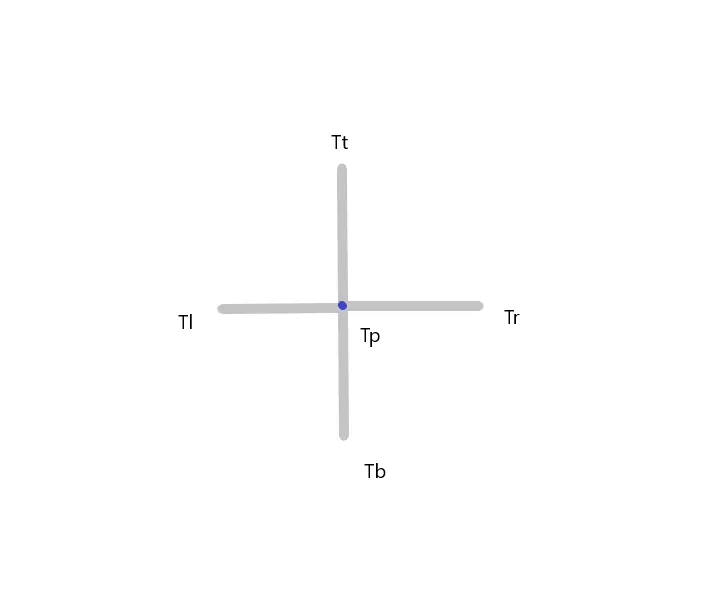
Discretizing the equation (1) we get ,
`T_p = 1/k [(T_L+T_R)/(trianglex^2) +(T_T+T_B)/(triangley^2)]`-----(2)
where k is `2((trianglex^2+triangley^2)/(trianglex^2triangley^2))`-------(3)
Since the computational domain is a square, `trianglex = triangley`
On further simplification, from equ 2 & equ 3, we get
`T_p = 0.25 [T_L+T_R +T_T+T_B]`
Main Program for Steady State :
clear all
close all
clc
%% Domain dimensions
nx =10;
ny=10;
L=1; % Length of the domain
B=1; % Breadth of domain
x = linspace(0,L,nx);
y = linspace(0,B,ny);
dx = x(2)-x(1);
dy = y(2)-y(1);
% Temperature guess values and boundary conditions
t = ones(nx,ny)*300;
t(1:end,1) = 400; %Left boundary
t(1:end,end) = 800; %Right boundary
t(1,1:end) = 600; %Top boundary
t(end,1:end) = 900; %Bottom boundary
%Temperature at the 4 corner of the rectangular boundary nodes
t(1,1) = (t(1,2)+t(2,1))/2;
t(1,end) = (t(1,end-1)+t(2,end))/2;
t(end,1) = (t((end-1),1)+t(end,2))/2;
t(end,end) = (t((end-1),end)+t(end,end-1))/2;
%Assigning the original values
t_initial = t;
told=t;
tol = 1e-4; % tolerance value with which error will be compared
alpha = 1.4; %Thermal diffusivity
omega = 1.2; %Relaxation factor for SOR method of iteration
%% For Steady state solution, calling respective function
[error_jb,iteration_jb] = jacobi_solver(nx,ny,dx,dy,t,told,tol);
[error_gs,iteration_gs] = gs_solver(nx,ny,dx,dy,t,told,tol);
[error_sor,iteration_sor] = sor_solver(nx,ny,dx,dy,t,told,tol,omega);
Function for Jacobi Solver :
function [error_jb,iteration_jb] = jacobi_solver(nx,ny,dx,dy,t,told,tol)
%% Initialising variable with intial values
iteration_jb=1;
error_jb= 9e9;
%% Convergence loop
while(error_jb>tol)
for i=2:nx-1
for j =2:ny-1
t(i,j) = 0.25*(told(i-1,j)+told(i+1,j)+told(i,j-1)+told(i,j+1));
end
end
error_jb = max(max(abs(told-t)));
told=t;
iteration_jb= iteration_jb+1;
end
%% Plotting the temperature profile
figure(1)
[C,h] = contourf(t);
colormap(jet);
clabel(C,h);
colorbar
set(gca, 'ydir','reverse')
xlabel('X axis')
ylabel('Y axis')
title('number of iterations for jacobian solver is ', iteration_jb);
end
OUTPUT
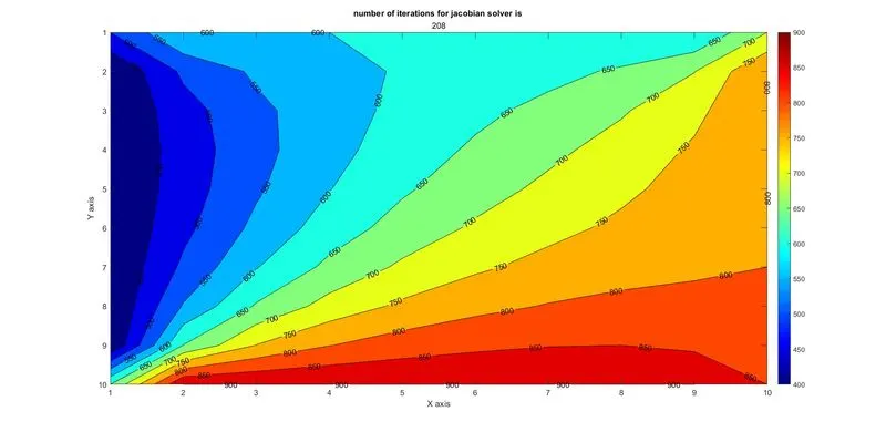
Function for Gauss Siedel Solver :
function [error_gs,iteration_gs] = gs_solver(nx,ny,dx,dy,t,told,tol)
%% Initialising variable with intial values
iteration_gs=1;
error_gs= 9e9;
%% Convergence loop
while(error_gs>tol)
for i=2:nx-1
for j =2:ny-1
t(i,j) = 0.25*(t(i-1,j)+told(i+1,j)+t(i,j-1)+told(i,j+1));
end
end
error_gs = max(max(abs(told-t)));
told=t;
iteration_gs= iteration_gs+1;
end
%% Plotting the temperature profile
figure(2)
[C,h] = contourf(t);
colormap(jet);
clabel(C,h);
colorbar
set(gca, 'ydir','reverse')
xlabel('X axis')
ylabel('Y axis')
title('number of iterations for gauss sidel solver is ', iteration_gs);
end
OUTPUT
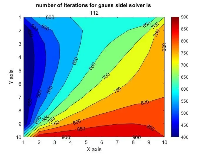
Function for SOR Solver :
function [error_sor,iteration_sor] = sor_solver(nx,ny,dx,dy,t,told,tol,omega)
%% Initialising variable with intial values
iteration_sor=1;
error_sor= 9e9;
%% Convergence loop
while(error_sor>tol)
for i=2:nx-1
for j =2:ny-1
t(i,j) = 0.25*(t(i-1,j)+told(i+1,j)+t(i,j-1)+told(i,j+1));
t(i,j) = told(i,j)*(1-omega) + omega*(t(i,j));
end
end
error_sor = max(max(abs(told-t)));
told=t;
iteration_sor= iteration_sor+1;
end
%% Plotting the temperature profile
figure(3)
[C,h] = contourf(t);
colormap(jet);
clabel(C,h);
colorbar
set(gca, 'ydir','reverse')
xlabel('X axis')
ylabel('Y axis')
title('number of iterations for SOR solver is ', iteration_sor);
end
OUTPUT
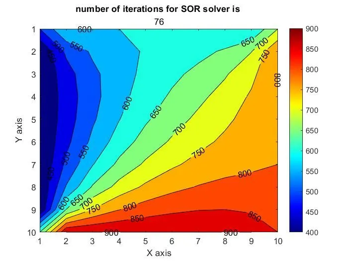
TRANSIENT STATE SOLUTION
Implicit Scheme :
`(delT)/(delt) = alpha((del^2T)/(trianglex^2) + (del^2T)/(triangley^2))`------(4)
On discretizing equ.(4), we get
`(T_p^(n+1)-T_p^n)/(trianglet) = alpha[(T_L-2T_P+T_R)/(trianglex^2) +(T_B-2T_P+T_T)/(triangley^2)]`
On further simplifying above equ. we get :
`T_p^(n+1) = 1/(1+k1+k2)(T_p^n+k1(T_L+T_R)^(n+1)+k2(T_B+T_T)^(n+1))`
where k1 = `alpha(trianglet)/(trianglex^2)` , k2=`alpha(trianglet)/(triangley^2)`
Explicit Scheme
`(delT)/(delt) = alpha((del^2T)/(trianglex^2) + (del^2T)/(triangley^2))`------(5)
On discretizing equ.(5), we get
`(T_p^(n+1)-T_p^n)/(trianglet) = alpha[(T_L-2T_P+T_R)/(trianglex^2) +(T_B-2T_P+T_T)/(triangley^2)]`
On further simplifying above equ. we get :
`T_p^(n+1) = T_p^n + k1(T_L-2T_P+T_R)^n +k2(T_B-2T_P+T_T)^n`
where k1 = `alpha(trianglet)/(trianglex^2)` , k2=`alpha(trianglet)/(triangley^2)`
-----------------------------------------------End of Theory---------------------------------------------------------------------------
Main Program for Transient State :
clear all
close all
clc
%% Domain dimensions
nx =10;
ny=10;
L=1; % Length of the domain
B=1; % Breadth of domain
x = linspace(0,L,nx);
y = linspace(0,B,ny);
dx = x(2)-x(1);
dy = y(2)-y(1);
% Temperature guess values and boundary conditions
t = ones(nx,ny)*300;
t(1:end,1) = 400; %Left boundary
t(1:end,end) = 800; %Right boundary
t(1,1:end) = 600; %Top boundary
t(end,1:end) = 900; %Bottom boundary
%Temperatur at the 4 corner of the rectangular boundary nodes
t(1,1) = (t(1,2)+t(2,1))/2;
t(1,end) = (t(1,end-1)+t(2,end))/2;
t(end,1) = (t((end-1),1)+t(end,2))/2;
t(end,end) = (t((end-1),end)+t(end,end-1))/2;
%Assigning the original values
t_initial = t;
told=t;
tol = 1e-4; % tolerance value with which error will be compared
alpha = 1.1; %Thermal diffusivity
omega = 1.1; %Relaxation factor for SOR method of iteration
%% For Transient state solution, calling respective function
[error_t,iteration_t] = unsteady_explicit(nx,ny,dx,dy,t,told,tol,alpha);
[error_jb_i,iteration_jb_i] = unsteady_implicit_jacobi(nx,ny,dx,dy,t,told,t_initial,tol,alpha);
[error_gs_i,iteration_gs_i] = unsteady_implicit_gs(nx,ny,dx,dy,t,told,t_initial,tol,alpha);
[error_sor_i,iteration_sor_i] = unsteady_implicit_sor(nx,ny,dx,dy,t,told,t_initial,tol,alpha,omega);
---------------------------------------------------------------------------------------------------------------------------------------
%Function for jacobi implicit scheme
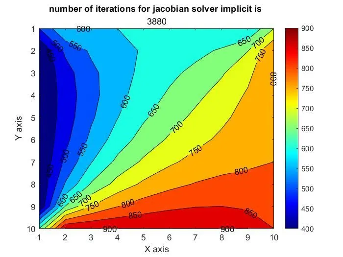
function [error_jb_imp,iteration_jb_imp] = unsteady_implicit_jacobi(nx,ny,dx,dy,t,told,t_initial,tol,alpha)
%% Initialising variable with intial values
iteration_jb_imp=1;
error_jb_imp= 9e9;
dt=1e-3;
k1 = dt*((alpha)/(dx^2));
k2 = dt*((alpha)/(dy^2));
term1 = 1/(1+(2*k1)+(2*k2));
term2 = k1*term1;
term3 = k2*term1;
%% Convergence loop
for m=1:1400
error_jb_imp =9e9;
while(error_jb_imp>tol)
for i=2:nx-1
for j =2:ny-1
TL = told(i-1,j);
TR = told(i+1,j);
TB = told(i,j-1);
TT = told(i,j+1);
H = TL+TR;
V = TB+TT;
t(i,j) = (t_initial(i,j)*term1) + (H*term2) + (V*term3);
end
end
error_jb_imp = max(max(abs(told-t)));
told = t;
iteration_jb_imp = iteration_jb_imp+1;
end
t_initial =t;
end
%% Plotting the temperature profile
figure(5)
[C,h] = contourf(t);
colormap(jet);
clabel(C,h);
colorbar
set(gca, 'ydir','reverse')
xlabel('X axis')
ylabel('Y axis')
title('number of iterations for jacobian solver implicit is ', iteration_jb_imp);
end
%Function for gauss sidel implicit scheme
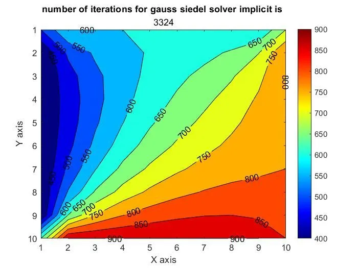
function [error_gs_imp,iteration_gs_imp] = unsteady_implicit_gs(nx,ny,dx,dy,t,told,t_initial,tol,alpha)
%% Initialising variable with intial values
iteration_gs_imp=1;
error_gs_imp= 9e9;
dt=1e-3;
k1 = (dt*alpha)/(dx^2);
k2 = (dt*alpha)/(dy^2);
term1 = (1+(2*k1)+(2*k2))^-1;
term2 = k1*term1;
term3 = k2*term1;
%% Convergence loop
for m=1:1400
error_gs_imp = 9e9;
while(error_gs_imp>tol)
for i=2:nx-1
for j =2:ny-1
TL = t(i-1,j);
TR = told(i+1,j);
TB = t(i,j-1);
TT = told(i,j+1);
H = TL+TR;
V = TB+TT;
t(i,j) = t_initial(i,j)*term1 + (term2*H) + (term3*V);
end
end
error_gs_imp = max(max(abs(told-t)));
told = t;
iteration_gs_imp = iteration_gs_imp+1;
end
t_initial =t;
end
%% Plotting the temperature profile
figure(6)
[C,h] = contourf(t);
colormap(jet);
clabel(C,h);
colorbar
set(gca, 'ydir','reverse')
xlabel('X axis')
ylabel('Y axis')
title('number of iterations for gauss siedel solver implicit is ', iteration_gs_imp);
end
%Function for SOR implicit scheme
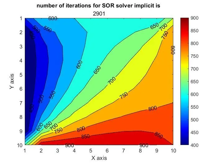
function [error_sor_imp,iteration_sor_imp] = unsteady_implicit_sor(nx,ny,dx,dy,t,told,t_initial,tol,alpha,omega)
%% Initialising variable with intial values
iteration_sor_imp=1;
error_sor_imp= 9e9;
dt=1e-3;
k1 = (dt*alpha)/(dx^2);
k2 = (dt*alpha)/(dy^2);
term1 = (1+(2*k1)+(2*k2))^-1;
term2 = k1*term1;
term3 = k2*term1;
%% Convergence loop
for m=1:1400
error_sor_imp=9e9;
while(error_sor_imp>tol)
for i=2:nx-1
for j =2:ny-1
TL = t(i-1,j);
TR = told(i+1,j);
TB = t(i,j-1);
TT = told(i,j+1);
H = TL+TR;
V = TB+TT;
t(i,j) = t_initial(i,j)*term1 + (term2*H) + (term3*V);
t(i,j) = told(i,j)*(1-omega) + t(i,j)*omega;
end
end
error_sor_imp = max(max(abs(told-t)));
told = t;
iteration_sor_imp = iteration_sor_imp+1;
end
t_initial =t;
end
%% Plotting the temperature profile
figure(7)
[C,h] = contourf(t);
colormap(jet);
clabel(C,h);
colorbar
set(gca, 'ydir','reverse')
xlabel('X axis')
ylabel('Y axis')
title('number of iterations for SOR solver implicit is ', iteration_sor_imp);
end
%Function for explicit scheme
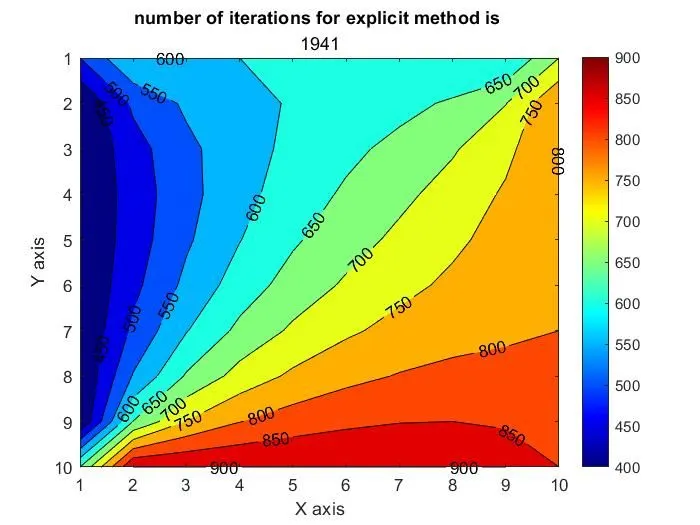
function [error_exp,iteration_exp] = unsteady_explicit(nx,ny,dx,dy,t,told,tol,alpha)
%% Initialising variable with intial values
iteration_exp=1;
error_exp= 9e9;
dt = 1e-3;
k1 = dt*alpha/dx^2;
k2 = dt*alpha/dy^2;
k3 = 1-(2*k1)-(2*k2);
%% Convergence loop
for m = 1:1400
error_exp =9e9;
while(error_exp>tol)
for i=2:nx-1
for j =2:ny-1
TL = told(i-1,j);
TR = told(i+1,j);
TB = told(i,j-1);
TT = told(i,j+1);
H = TL+TR;
V = TB+TT;
t(i,j) = told(i,j)*k3 + (k1*H) + (k2*V);
end
end
error_exp = max(max(abs(told-t)));
iteration_exp = iteration_exp+1;
told =t;
end
end
%% Plotting the temperature profile
figure(4)
[C,h] = contourf(t);
colormap(jet);
clabel(C,h);
colorbar
set(gca, 'ydir','reverse')
xlabel('X axis')
ylabel('Y axis')
title('number of iterations for explicit method is ', iteration_exp);
end
Explanation of Results
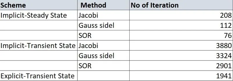
1) Considering all the scheme and the respective iterative method followed, no of iteration in the increasing order is SOR<Gauss Sidel<Jacobi
2)SOR is the most effective since it took lesser no of iteration for the results to converge.
3) Steady state takes lesser no of iteration for convergence compared to unsteady state.
4) Explicit transient scheme achieves convergence in lesser iteration compared to implicit transient schemes.