Week 3.5 - Deriving 4th order approximation of a 2nd order derivative using Taylor Table method

Objective : To derive the fourth order approximations of second order derivative using the taylor table method.

1) Central Difference Scheme : In this method, we take nodes symmetrical about the main node. For calculating the no of nodes to be taken we can use the formula given as :

p+q-1, where p is the order of the derivative & q is the order of approximation

Therefore no of nodes in this method = 2+4-1=5

`(del^2f)/(delx^2) =` af(i-2) + bf(i-1) + cf(i) + df(i+1) + ef(i+2) ------>(1)

	f(i)	dxf'(i)	`dx^2f''(i)`	`dx^3f'''(i)`	`dx^4f''''(i)`	`dx^5f'''''(i)`
af(i-2)	a	-2a	4a/2	-8a/6	16a/24	-32a/120
bf(i-1)	b	-b	b/2	-b/6	b/24	-b/120
cf(i)	c	0	0	0	0	0
df(i+1)	d	d	d/2	d/6	d/24	d/120
ef(i+2)	e	2e	4e/2	8e/6	16e/24	32e/120
sum of coefficients	0	0	1	0	0	0

This table can be transformed to a form : AX=B

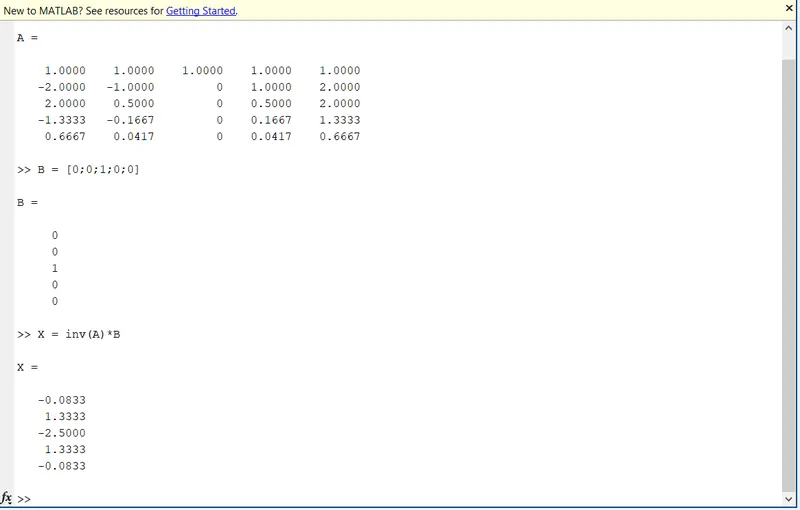
Therefore value of coefficients are : a =-0.0833,b=1.3333,c=-2.5,d=1.3333,e=-0.0833

2) Skewed right sided difference : If we are not knowing the values of a function at the left hand side nodes then we use this method. The no of nodes to be taken can be found out by the formula : p +q where p is the order of the derivative & q is the order of approximation

So, no of nodes = 2+4 = 6

`(del^2f)/(delx^2) =` af(i) + bf(i+1) + cf(i+2) + df(i+3) + ef(i+4) + ff(i+5) ------>(2`

	f(x)	dxf'(x)	`dx^2f''(x)`	`dx^3f'''(x)`	`dx^4f''''(x)`	`dx^5f'''''(x)`
af(i)	a	0	0	0	0	0
bf(i+1)	b	b	b/2	b/6	b/24	b/120
cf(i+2)	c	2c	4c/2	8c/6	16c/24	32c/120
df(i+3)	d	3d	9d/2	27d/6	81d/24	243d/120
ef(i+4)	e	4e	16e/2	64e/6	256e/24	1024e/120
ff(i+5)	f	5f	25f/2	125f/6	625f/24	3125f/120
Sum of coefficients	0	0	1	0	0	0

This table can be transformed to a form : AX=B

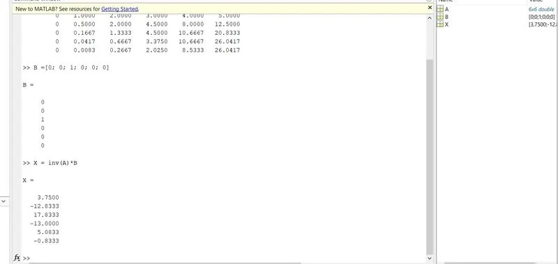
Therefore value of coefficients are : a=3.75,b=-12.8333,c=17.8333,d=-13.0000,e=5.0833,f=-0.8333

3) Skewed left sided difference :

If we are not knowing the values of a function at the right hand side nodes then we use this method. The no of nodes to be taken can be found out by the formula : p +q where p is the order of the derivative & q is the order of approximation

So, no of nodes = 2+4 = 6

`(del^2f)/(delx^2) =` af(i-5) + bf(i-4) + cf(i-3) + df(i-2) + ef(i-1) + ff(i)`-------> (3)

	f(x)	dxf'(x)	`dx^2f''(x)`	`dx^3f'''(x)`	`dx^4f''''(x)`	`dx^5f'''''(x)`
af(i-5)	a	-5a	25a/2	-125a/6	625a/24	-3125a/120
bf(i-4)	b	-4b	16b/2	-64b/6	256b/24	-1024b/120
cf(i-3)	c	-3c	9c/2	-27c/6	81c/24	-243c/120
df(i-2)	d	-2d	4d/2	-8d/6	16d/24	-32d/120
ef(i-1)	e	-1e	e/2	-e/6	e/24	-e/120
ff(i)	f	0	0	0	0	0
Sum of coefficients	0	0	1	0	0	0

This table can be transformed to a form : AX=B

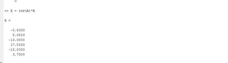
Therefore value of coefficients are : a =-0.8333,b=5.0833,c=-13.0000,d=17.8333,e=-12.8333,f=3.7500

-------------------------------------------------------------------------------------------------------------------------------------------

Matlab Program

clear all
close all
clc

%% Input values for calculating the function value for different range of dx
x=pi/3;

dx = linspace(pi/4,pi/4000,30);
Analytical_function = exp(x)*cos(x);
Analytical_second_Derv= -2*(exp(x)*sin(x));
%% for loop to iterate through dx values
central_diff_error = zeros(1,length(dx));
skewed_right_error = zeros(1,length(dx));
skewed_left_error = zeros(1,length(dx));

for i=1:length(dx)
central_diff_error(i) = fourth_order_cds(x,dx(i));
skewed_right_error(i) = fourth_order_skr(x,dx(i));
skewed_left_error(i) = fourth_order_skl(x,dx(i));
end

%% Plotting the different schemers error calculation w.r.t to range of dx values

figure(1)
loglog(dx,central_diff_error,'linewidth',2,'color','r')
hold on
loglog(dx,skewed_right_error,'linewidth',2,'color','b')
hold on
loglog(dx,skewed_left_error,'linewidth',2 ,'color','g')
xlabel('Range of dx')
ylabel('Error for different schemes')
legend('central diff error','skewed right error','skewed left error')
title('Schemes Error vs Range of dx values')

Function for central difference scheme

function central_diff_Er = fourth_order_cds(x,dx)

%% for central difference scheme we know that, (del^2f)/(delx^2) =` af(i-2) + bf(i-1) + cf(i) + df(i+1) + ef(i+2)/dx^2...
a =-0.0833;b=1.3333;c=-2.5000;d=1.3333;e=-0.0833; %from derivation
Analytical_second_Derv= -2*(exp(x)*sin(x));

central_diff = (((a)*(exp(x-(2*dx))*cos(x-(2*dx)))) +((b)*(exp(x-dx)*cos(x-dx)))+((c)*(exp(x)*cos(x))) + ((d)*(exp(x+dx)*cos(x+dx)))+((e)*(exp(x+(2*dx))*cos(x+(2*dx)))))/(dx^2);
central_diff_Er = abs(central_diff - Analytical_second_Derv);
end

Function for skewed right sided scheme

function skr_diff_Er = fourth_order_skr(x,dx)

%% for skewed right sided scheme, (del^2f)/(delx^2) =` af(i) + bf(i+1) + cf(i+2) + df(i+3) + ef(i+4) + ff(i+5)/dx^2
a=3.75;b=-12.8333;c=17.8333;d=-13.0000;e=5.0833;f=-0.8333; %from derivation

Analytical_second_Derv= -2*(exp(x)*sin(x));
skewed_right = ((a)*(exp(x)*cos(x)) +(b)*(exp(x+dx)*cos(x+dx))+(c)*(exp(x+(2*dx))*cos(x+(2*dx))) + (d)*(exp(x+(3*dx))*cos(x+(3*dx)))+(e)*(exp(x+(4*dx))*cos(x+(4*dx)))+(f)*(exp(x+(5*dx))*cos(x+(5*dx))))/(dx^2);
skr_diff_Er = abs(skewed_right-Analytical_second_Derv);
end

Function for skewed left sided scheme

function skewed_left_Err = fourth_order_skl(x,dx)

%% for skewed left sided scheme, (del^2f)/(delx^2) =` af(i-5) + bf(i-4) + cf(i-3) + df(i-2) + ef(i-1) + ff(i)/dx^2
a =-0.8333;b=5.0833;c=-13.0000;d=17.8333;e=-12.8333;f=3.7500; % from derivation

Analytical_second_Derv= -2*(exp(x)*sin(x));
skewed_left = ((a)*(exp(x-(5*dx))*cos(x-(5*dx))) +(b)*(exp(x-(4*dx))*cos(x-(4*dx)))+(c)*(exp(x-(3*dx))*cos(x-(3*dx))) + (d)*(exp(x-(2*dx))*cos(x-(2*dx)))+(e)*((exp(x-dx))*cos(x-dx))+(f)*((exp(x)*cos(x))))/(dx^2);
skewed_left_Err = abs(skewed_left-Analytical_second_Derv);

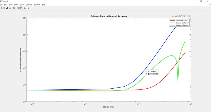
Results Explanation

1) From the above plot we can say that , for central difference scheme error values is less compared to skewed right and left scheme.

2) For problems where, numerical approximation for boundary or corner is to be evaluated then we cannot use central difference scheme for it. In that situation skewed schemes are used as data from one side of node is available.