Week 5.1 - Mid term project - Solving the steady and unsteady 2D heat conduction problem
1. Introduction, simulation setup
The program is structured in three files: "main.m", "data.m", "plotResults.m", with straightforward meanings.
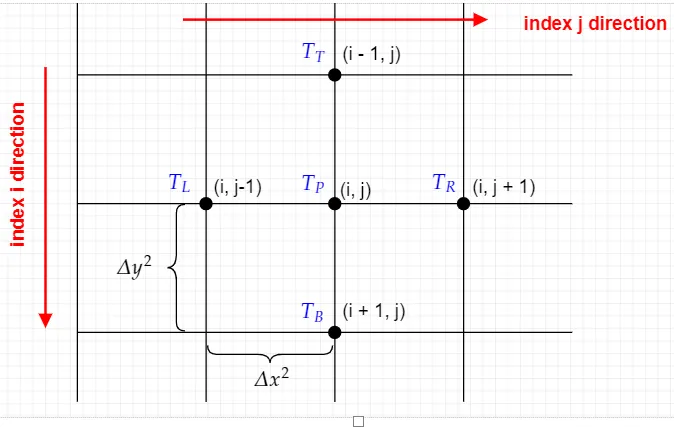
The convention used for indexing the mesh grid throughout the code is a little bit different from the one used in the lessons and in the hint. The final result displayed in the "ASSIGNMENT HELP VIDEO PART-2" is nevertheless similar.
With "i" it is denoted the row index, while with "j" it is denoted the column index.
This is because I wanted to follow the same indexing rules within Matlab. It was easier for me to display the temperature grid matrix in the Command Window and to debug the code.
I hope this will not create confusion.
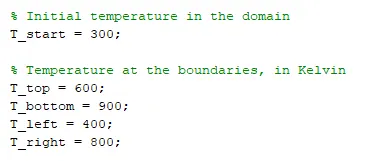
Here after it is displayed the initial condition; the temperature inside the domain is set at 300K.
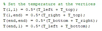
The temperature at the corners is the average between the temperatures at the sides:
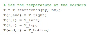
Graphically, the temperature matrix (namely, the "T" variable) has the same shape of the topology of our problem:
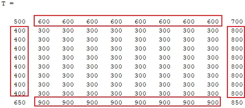
We need to define the error tolerance, and a default error value:
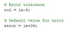
The mesh grid size is 11x11.
The domain is 1mx1m, and the thermal diffusivity term is set to be 0.1m^2/s, which is an extremely high value, therefore the solution converges rapidly.
2. 2D Steady-State Heat Conduction Problem
A convergence loop is needed in order to solve this particular problem, but not a time marching loop. Below the convergence loop, two nested space loops have been used in order to solve the equations in directions left-right and top-bottom.
Let's discretize the second-order linear equation:
`(del^2T)/(del x^2) + (del^2 T)/(del y^2) = 0`
`(T_L - 2T_P + T_R)/(Delta x^2) + (T_T- 2T_P + T_B)/(Delta y^2)=0`
`2/(Delta x^2)T_P + 2/(Delta y^2)T_P = (T_L+T_R)/(Delta x^2) + (T_T+T_B)/(Delta y^2)`
`2(Delta x^2 + Delta y^2)/(Delta x^2 Delta y^2) T_P = (T_L+T_R)/(Delta x^2) + (T_T+T_B)/(Delta y^2)`
Let's assume:
`k = 2(Delta x^2 + Delta y^2)/(Delta x^2 Delta y^2)`
We can write:
`T_P = (T_L+T_R)/(k Delta x^2) + (T_T+T_B)/(k Delta y^2)`
The difference between the Jacobi and the Gauss-Seidel method for computing the temperature at one point is whether to use the newly computed values of temperature on the left side and on the top side of the grid, or to still use the values computed in the previous iteration.
Jacobi method:
`T_P^("(new)") = (T_L^("(old)")+T_R^("(old)"))/(k Delta x^2) + (T_T^("(old)")+T_B^("(old)"))/(k Delta y^2)`
Gauss-Seidel method:
`T_P^("(new)") = (T_L^("(new)")+T_R^("(old)"))/(k Delta x^2) + (T_T^("(new)")+T_B^("(old)"))/(k Delta y^2)`
The right and the bottom temperatures are not yet computed, therefore we keep the values obtained in the previous iteration.
SOR method
The equation implemented for the SOR method is as follows:
`T_P^("(new)") = (1 - omega) T_P^("(old)") + omega [(T_L^("(new)")+T_R^("(old)"))/(k Delta x^2) + (T_T^("(new)")+T_B^("(old)"))/(k Delta y^2)]`
The iteration (while loop) stops when the condition:
`max(|T^("(new)")-T^("(old)")|)<"tolerance"`
is reached.
3. Transient Heat Conduction Problem
In this problem, a time-marching loop is needed above the convergence loop.
The following methods are intended to discretize and solve the following second-order differential equation:
`(del T)/(del t) = alpha((del^2 T)/(del x^2) + (del^2 T)/(del y^2))`
In all the following implicit methods, the RHS of the equation is calculated at the same time step n+1
`(T_P^(n+1) - T_P^(n))/(Delta t) = alpha[ (T_L^(n+1) - 2T_P^(n+1) + T_R^(n+1))/(Delta x^2) + (T_T^(n+1)- 2T_P^(n+1) + T_B^(n+1))/(Delta y^2)]`
3.1. Transient Heat Conduction Equation - Implicit Jacobi
We reorder the terms of the previous equation, bringing only `T_P^(n+1)` to the left side, and multiplying both terms by Delta t:
`T_P^(n+1) + 2 (alpha Delta t)/(Delta x^2) T_P^(n+1) + 2 (alpha Delta t)/(Delta y^2) T_P^(n+1) = T_P^n + (alpha Delta t)/(Delta x^2) (T_L^n + T_R^n) + (alpha Delta t)/(Delta y^2) (T_T^n + T_B^n)`
Let's make the same assumptions of the hint:
`k_1=(alpha*Delta t)/(Deltax^2)`
`k_2=(alpha*Delta t)/(Delta y^2)`
`"term1"=1/(1 + 2k_1 + 2k_2)`
`"term2"=k_1*"term1"`
`"term3"=k_2*"term1"`
`H=T_L+T_R`
`V=T_T+T_B`
Therefore the equation to solve simplifies in the following:
`T_P^(n-1)="term1"*T_P^N+"term2"*H+"term3"*V`
An analogous approach has been used for the GS and SOR methods, considering the points already discussed for the steady-state solution.
3.4. Explicit 2D Transient Heat Conduction Equation
The equation:
`(del T)/(del t) = alpha((del^2T)/(del x^2) + (del^2 T)/(del y^2))`
is discretized as follows:
`(T_P^(n+1) - T_P^(n))/(Delta t) = alpha[ (T_L^(n) - 2T_P^(n) + T_R^(n))/(Delta x^2) + (T_T^(n)- 2T_P^(n) + T_B^(n))/(Delta y^2)]`
`T_P^(n+1) = T_P^(n) + alpha Delta t[(T_L^(n) - 2T_P^(n) + T_R^(n))/(Delta x^2) + (T_T^(n)- 2T_P^(n) + T_B^(n))/(Delta y^2)]`
No iterative solvers are needed in this case, because all the terms on the RHS of the equations are known.
We only need to pay attention to the terms:
`k_1 = (alpha Delta t)/(Delta x^2); qquad k_2 = (alpha Delta t)/(Delta y^2)`
If `k_1+k_2>0.5`, the solution will be unstable. This represents the CFL criteria.
Plots and results
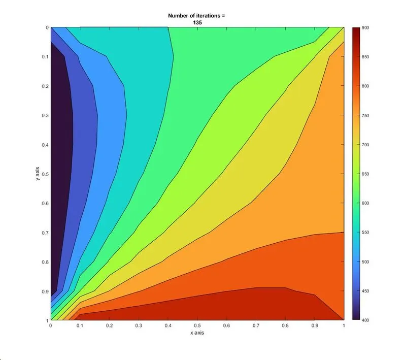
An example of plot obtained is shown below. In particular, this is the Gauss-Seidel steady-state solution, which converges after 135 iterations.
%
%  File     :   main.m
%
%  Author   :   Matteo Agositnone
%  Date     :   09.10.2021
%
%  Course   :   SKILL-LYNC - Introduction to CFD using MATLAB and OpenFOAM
%
%  Challenge: Week 5.1 - Mid term project - Solving the steady and unsteady 2D heat conduction problem

clearvars
close all
clc

% Introductory stuff displayed
fprintf('Week 5.1 - Mid term project - Solving the steady and unsteady 2D heat conduction problem \nby Matteo Agostinone\n\n')

%% SECTION 1: DEFINE DATA
%  All the input data is collected to a separate file "data.m", and loaded
%  here
data

% Write on the terminal the temperature at the borders
direction = ["top";"bottom";"left";"right"];
temperature = num2str([T_top; T_bottom; T_left; T_right]);

disp(strcat("The temperature at the ", direction, " boundary is ", temperature, ' K'))

% The program allows the user to choose whether to solve
% the steady-state problem rather than the transient problem
problem = input([
    'Would you like to solve the steady-state or the transient problem?',...
    '\n1 = Steady state; 2 = Transient',...
    '\n'
    ]);

%% SECTION 2: INITIAL CONDITIONS

% Build the mesh
x = linspace(0, Lx, nx);
y = linspace(0, Ly, ny);
[X,Y] = meshgrid(x, y);

dx = Lx/(nx - 1);
dy = Ly/(ny - 1);

% Set the temperature at the borders
T = T_start*ones(ny, nx);
T(:,end) = T_right;
T(:,1) = T_left;
T(1,:) = T_top;
T(end,:) = T_bottom;

% Set the temperature at the vertices
T(1,1) = 0.5*(T_left + T_top);
T(1,end) = 0.5*(T_right + T_top);
T(end,end) = 0.5*(T_bottom + T_right);
T(end,1) = 0.5*(T_left + T_bottom);

% Set the initial temperature
T_initial = T;

% Set the temperature values that will update at each space loop iteration
T_old = T;

% Set an iteration counter
counter = 0;

%% SECTION 3: RUN THE SIMULATION

if problem == 1
    %% SECTION 3.1: STEADY STATE PROBLEM

    % This is a factor that goes into the 2nd order differential equations,
    % as shown in the hint of this problem
    k = 2*(dx^2 + dy^2)/(dx^2*dy^2);

    % Method selection
    % 1 = Jacobi, 2 = Gauss-Seidel, 3 = OR
    method = input([
        'Select a method for the iterative solver',...
        '\n1 = Jacobi, 2 = Gauss-Seidel, 3 = Successive Over-relaxation',...
        '\n'
        ]);

    if method == 1
        %% SECTION 3.1.1: JACOBI METHOD FOR STEADY STATE PROBLEM

        % Outer iteration loop
        while error > tol

            % Space loop
            for i = 2 : ny - 1 % We are proceeding from top to bottom
                for j = 2 : nx - 1 % We are proceeding from left to right

                    T(i,j) = 1/k*(T_old(i,j-1) + T_old(i,j+1))/dx^2 + 1/k*(T_old(i-1,j) + T_old(i+1,j))/dy^2;

                end
            end

            error = max(abs(T - T_old), [], 'all');

            % Update T_old
            T_old = T;

            % Update the counter
            counter = counter + 1;

        end

            % Plot results
            plotResults

    elseif method == 2
        %% SECTION 3.1.2 GAUSS-SEIDEL METHOD FOR STEADY STATE EQUATION

        % Outer iteration loop
        while error > tol

            % Space loop
            for i = 2 : ny - 1 % We are proceeding from top to bottom
                for j = 2 : nx - 1 % We are proceeding from left to right

                    T(i,j) = 1/k*(T(i,j-1) + T_old(i,j+1))/dx^2 + 1/k*(T(i-1,j) + T_old(i+1,j))/dy^2;

                end
            end

            error = max(abs(T - T_old), [], 'all');

            % Update T_old
            T_old = T;

            % Update the counter
            counter = counter + 1;

        end

        % Plot results
        plotResults

    elseif method == 3
        %% SECTION 3.1.3: SUCCESSIVE OVER RELAXATION METHOD FOR STEADY STATE PROBLEM

            % Outer iteration loop
        while error > tol

            % Space loop
            for i = 2 : ny - 1 % We are proceeding from top to bottom
                for j = 2 : nx - 1 % We are proceeding from left to right

                    T(i,j) = (1 - relax_factor)*T_old(i,j) + relax_factor*(1/k*(T(i,j-1) + T_old(i,j+1))/dx^2 + 1/k*(T(i-1,j) + T_old(i+1,j))/dy^2);

                end
            end

            error = max(abs(T - T_old), [], 'all');

            % Update T_old
            T_old = T;

            % Update the counter
            counter = counter + 1;

        end

        % Plot results
        plotResults

    else
        disp('Wrong input')
    end
elseif problem == 2
%% SECTION 3.2: TRANSIENT PROBLEM

% Following the hint terminology:
k1 = alpha*dt/dx^2;
k2 = alpha*dt/dy^2;

term1 = (1 + 2*k1 + 2*k2)^(-1);
term2 = k1*term1;
term3 = k2*term1;

% Initialezing T_prev_dt, which will be used inside the time loop, and it
% will remain constant inside the space loop
T_prev_dt = T;

method = input([
        'Select a method for the iterative solver',...
        '\n1 = Jacobi, 2 = Gauss-Seidel, 3 = Successive Over-relaxation, 4 = Explicit',...
        '\n'
        ]);
    if method == 1

        %% SECTION 3.2.1: JACOBI METHOD FOR TRANSIENT PROBLEM

    % Time loop
    for nt = 1:1000

        % Convergence loop
        while error > tol

            % Space loop
                for i = 2 : ny - 1 % We are proceeding from the top to the bottom of the matrix
                    for j = 2 : nx - 1 % We are proceeding from the left to the right of the matrix

                        H = T_old(i,j-1) + T_old(i,j+1);
                        V = T_old(i-1,j) + T_old(i+1,j);

                        T(i,j) = term1*T_prev_dt(i,j) + term2*H + term3*V;

                    end
                end

                % Compute the error
                error = max(abs(T - T_old), [], 'all');
                % Update the T_old matrix for next convergence iteration
                T_old = T;
        end

        % Update the T_prev_dt matrix for next time iteration
        T_prev_dt = T;

        % Reset the error to the default value
        error = 1e+09;

        % Update the counter
        counter = counter + 1;

        % Plot results
        plotResults

        pause(0.001)

    end % Time loop, method 1, problem 2

    elseif method == 2

        %% SECTION 3.2.2: GAUSS-SEIDEL METHOD FOR TRANSIENT PROBLEM

        % Time loop
        for nt = 1:1000

            % Convergence loop
            while error > tol

                % Space loop
                    for i = 2 : ny - 1 % We are proceeding from the top to the bottom of the matrix
                        for j = 2 : nx - 1 % We are proceeding from the left to the right of the matrix

                            H = T(i,j-1) + T_old(i,j+1);
                            V = T(i-1,j) + T_old(i+1,j);

                            T(i,j) = term1*T_prev_dt(i,j) + term2*H + term3*V;

                        end
                    end

                    % Compute the error
                    error = max(abs(T - T_old), [], 'all');
                    % Update the T_old matrix for next convergence iteration
                    T_old = T;
            end

            % Update the T_prev_dt matrix for next time iteration
            T_prev_dt = T;

            % Reset the error to the default value
            error = 1e+09;

            % Update the counter
            counter = counter + 1;

            % Plot results
            plotResults

            pause(0.001)

        end % Time loop, method 2, problem 2

    elseif method == 3
        %% SECTION 3.2.3: SUCCESSIVE OVER-RELAXATION METHOD FOR TRANSIENT PROBLEM

        % Time loop
        for nt = 1:1000

            % Convergence loop
            while error > tol

                % Space loop
                    for i = 2 : ny - 1 % We are proceeding from the top to the bottom of the matrix
                        for j = 2 : nx - 1 % We are proceeding from the left to the right of the matrix

                            H = T(i,j-1) + T_old(i,j+1);
                            V = T(i-1,j) + T_old(i+1,j);

                            T(i,j) = (1 - relax_factor)*T_old(i,j) + relax_factor*(term1*T_prev_dt(i,j) + term2*H + term3*V);

                        end
                    end

                    % Compute the error
                    error = max(abs(T - T_old), [], 'all');
                    % Update the T_old matrix for next convergence iteration
                    T_old = T;
            end

            % Update the T_prev_dt matrix for next time iteration
            T_prev_dt = T;

            % Reset the error to the default value
            error = 1e+09;

            % Update the counter
            counter = counter + 1;

            % Plot results
            plotResults

            pause(0.01)

        end % Time loop, method 2, problem 2
    elseif method == 4
        %% SECTION 3.2.4: EXPLICIT SOLUTION

        % CFL numbers
        k1 = alpha*dt/dx^2;
        k2 = alpha*dt/dy^2;

        % Time loop
        for nt = 1:1000

            % Space loop
            for i = 2 : ny - 1 % We are proceeding from the top to the bottom of the matrix
                for j = 2 : nx - 1 % We are proceeding from the left to the right of the matrix

                    T(i,j) = T_old(i,j) + k1*(T_old(i,j-1) - 2*T_old(i,j) + T_old(i,j+1)) + k2*(T_old(i-1,j) - 2*T_old(i,j) + T_old(i+1,j));

                end % for j
            end % for i

            T_old = T;

            % Update the counter
            counter = counter + 1;

            % Plot results
            plotResults

            pause(0.01)

        end % Time loop

    else
        disp('Wrong input')
    end % method choice of transient solution
else

    disp("Wrong input")

end % of the program
%
% File : data.m
%
% Author : Matteo Agositnone
% Date : 09.10.2021
%
% Course : SKILL-LYNC - Introduction to CFD using MATLAB and OpenFOAM
%
% Challenge: Week 5.1 - Mid term project - Solving the steady and unsteady 2D heat conduction problem
% This script collects all the data for solving the problem
% Temperature at the boundaries, in Kelvin
T_top = 600;
T_bottom = 900;
T_left = 400;
T_right = 800;
% Length of the domain along x and y, in meters
Lx = 1;
Ly = 1;
% Mesh grid
nx = 11;
ny = 11;
% Initial temperature in the domain, in K
T_start = 300;
% Error tolerance
tol = 1e-4;
% Default value for error
error = 1e+09;
% Relaxation factor (for SOR iterative method)
relax_factor = 1.2;
% Transient delta t
dt = 0.01;
% Thermal diffusivity, m^2/s
alpha = 0.1;%
% File : plotResults.m
%
% Author : Matteo Agositnone
% Date : 09.10.2021
%
% Course : SKILL-LYNC - Introduction to CFD using MATLAB and OpenFOAM
%
% Challenge: Week 5.1 - Mid term project - Solving the steady and unsteady 2D heat conduction problem
% Plot results
contourf(x,y,T)
set(gca,'Ydir','reverse')
axis equal
colormap turbo;
set(gcf, 'Position', get(0, 'Screensize'));
title({
'Number of iterations = ' num2str(counter)
})
xlabel('x axis')
ylabel('y axis')
zlabel('temperature in Kelvin')
colorbar