Week 3.5 - Deriving 4th order approximation of a 2nd order derivative using Taylor Table method
The second-order derivative of:
`f(x)=e^(x)cosx`
is:
`f''(x)=-2e^(x)sinx`
This is the expression that we would like to compare with our difference schemes.
Symmetric difference scheme
Let's start to derive an expression for a symmetric scheme of the fourth-order approximation of the second-order derivative.
How many points in the stencil should we get? By following the equation in the HINT i), we can write:
`P=N-Q+1 qquad => qquad N=P+Q-1 quad, qquad qquad P=4, quad Q=2`
hence `N = 5`
Now, we are looking for an expression of the second-order derivative `f''(x)`, calculated at `x = i` of this form:
`(delta^2 f)/(delta x^2) = (a f_(i-2)+b f_(i-1)+c f_i+df_(i+1)+ef_(i+2))/(Delta x)^2 qquad qquad qquad (1)`
where:
- `(delta^2 f)/(delta x^2)` is the approximated second-order derivative, distinguished from `(d^2 f)/(d x^2)` which is the analytical expression
- `f_(i-2)=f(i-2 Delta x), quad f_(i-1)=f(i-Delta x)` and so on, where `Delta x` is a arbritrary chosen small interval
By taking five points, the equation of HINT i) ensures us that we are evaluating a fourth-order approximation.
Let's now write down the fourth-order approximations of the terms `f_(i+k)` in the equation (1):
`af_(i-2) = a[ f(i) - 2Delta xf'(i) +(4(Delta x)^2)/(2!)f''(i) - (8(Delta x)^3)/(3!)f'''(i) + (16(Delta x)^4)/(4!)f^(IV)(i)]`
`bf_(i-1) = b[ f(i) - Delta xf'(i) +((Delta x)^2)/(2!)f''(i) - ((Delta x)^3)/(3!)f'''(i) + ((Delta x)^4)/(4!)f^(IV)(i)]`
`cf_i = c f(i)`
`df_(i+1) = d[ f(i) + Delta xf'(i) +((Delta x)^2)/(2!)f''(i) + ((Delta x)^3)/(3!)f'''(i) + ((Delta x)^4)/(4!)f^(IV)(i)]`
`ef_(i+2) = e[ f(i) + 2Delta xf'(i) +(4(Delta x)^2)/(2!)f''(i) + (8(Delta x)^3)/(3!)f'''(i) + (16(Delta x)^4)/(4!)f^(IV)(i)]`
From those equations we can write down the following Taylor's table:
| `f(i)` | `Delta x f'(i)` | `(Delta x)^2 f''(i)` | `(Delta x)^3f'''(i)` | `(Deltax)^4f^(IV)(i)` | |
| `af_(i-2)` | `a` | `-2a` | `2a` | `-4/3a` | `2/3a` |
| `bf_(i-1)` | `b` | `-b` | `1/2b` | `-1/6b` | `1/24b` |
| `cf_i` | `c` | `0` | `0` | `0` | `0` |
| `df_(i+1)` | `d` | `d` | `1/2d` | `1/6d` | `1/24d` |
| `ef_(i+2)` | `e` | `2e` | `2e` | `4/3e` | `2/3e` |
| `0` | `0` | `1` | `0` | `0` |
which leads to the following system of equations:
`{(a,+b,+c,+d,+e,=,0),(-2a,-b,+0c, +d,+2e,=,0),(2a,+1/2b,+0c, +1/2d,+2e,=,1),(-4/3a,-1/6b,+0c, +1/6d,+4/3e,=,0),(2/3a,+1/24b,+0c, +1/24d,+2/3e,=,0):}`
This can be written in a matrix form:
`[[1, 1, 1, 1, 1],[-2,-1,0,1,2],[2,1/2,0,1/2,2],[-4/3,-1/6,0,1/6,4/3],[2/3,1/24,0,1/24,2/3]] [[a],[b],[c],[d],[e]] = [[0],[0],[1],[0],[0]]`
`AX=B qquad qquad Rightarrow qquad qquad X=A^(-1)B`
We have finally got the five coefficients we need! We just need to implemet Equation 1) in Matlab and find the difference with the analytical derivative.
Skewed difference scheme
How many points in the stencil should we get? By following the equation in the HINT ii), we can write:
`P=N-Q qquad => qquad N=P+Q quad, qquad qquad P=4, quad Q=2`
hence `N = 6`
Now, we are looking for an expression of the second-order derivative `f''(x)`, calculated at `x = i` of this form:
`(delta^2 f)/(delta x^2) = (a f_(i)+b f_(i+1)+c f_(i+2)+df_(i+3)+ef_(i+4)+gf_(i+5))/(Delta x)^2 qquad qquad qquad (2)`
for right-sided scheme, and:
`(delta^2 f)/(delta x^2) = (a f_(i)+b f_(i-1)+c f_(i-2)+df_(i-3)+ef_(i-4)+gf_(i-5))/(Delta x)^2 qquad qquad qquad (3)`
for left-sided scheme.
By taking six points, the equation of HINT ii) ensures us that we are evaluating a fourth-order approximation.
Let's now write down the fourth-order approximations of the terms `f_(i+k)` in the equation (2):
`af_i=af(i)`
`bf_(i+1) = b[ f(i) + Delta xf'(i) +((Delta x)^2)/(2!)f''(i) + ((Delta x)^3)/(3!)f'''(i) + ((Delta x)^4)/(4!)f^(IV)(i) + ((Delta x)^5)/(5!)f^(V)(i)]`
`cf_(i+2) = c[ f(i) + 2Delta xf'(i) +(4(Delta x)^2)/(2!)f''(i) + (8(Delta x)^3)/(3!)f'''(i) + (16(Delta x)^4)/(4!)f^(IV)(i) + (32(Delta x)^5)/(5!)f^(V)(i)]`
`df_(i+3) = d[ f(i) + 3Delta xf'(i) +(3^2(Delta x)^2)/(2!)f''(i) + (3^3(Delta x)^3)/(3!)f'''(i) + (3^4(Delta x)^4)/(4!)f^(IV)(i) + (3^5(Delta x)^5)/(5!)f^(V)(i)]`
`ef_(i+4) = e[ f(i) + 4Delta xf'(i) +(4^2(Delta x)^2)/(2!)f''(i) + (4^3(Delta x)^3)/(3!)f'''(i) + (4^4(Delta x)^4)/(4!)f^(IV)(i) + (4^5(Delta x)^5)/(5!)f^(V)(i)]`
`gf_(i+4) = g[ f(i) + 5Delta xf'(i) +(5^2(Delta x)^2)/(2!)f''(i) + (5^3(Delta x)^3)/(3!)f'''(i) + (5^4(Delta x)^4)/(4!)f^(IV)(i) + (5^5(Delta x)^5)/(5!)f^(V)(i)]`
and in the equation (3):
`af_i=af(i)`
`bf_(i-1) = b[ f(i) - Delta xf'(i) +((Delta x)^2)/(2!)f''(i) - ((Delta x)^3)/(3!)f'''(i) + ((Delta x)^4)/(4!)f^(IV)(i) - ((Delta x)^5)/(5!)f^(V)(i)]`
`cf_(i-2) = c[ f(i) - 2Delta xf'(i) +(4(Delta x)^2)/(2!)f''(i) - (8(Delta x)^3)/(3!)f'''(i) + (16(Delta x)^4)/(4!)f^(IV)(i) - (32(Delta x)^5)/(5!)f^(V)(i)]`
`df_(i-3) = d[ f(i) - 3Delta xf'(i) +(3^2(Delta x)^2)/(2!)f''(i) - (3^3(Delta x)^3)/(3!)f'''(i) + (3^4(Delta x)^4)/(4!)f^(IV)(i) - (3^5(Delta x)^5)/(5!)f^(V)(i)]`
`ef_(i-4) = e[ f(i) - 4Delta xf'(i) +(4^2(Delta x)^2)/(2!)f''(i) - (4^3(Delta x)^3)/(3!)f'''(i) + (4^4(Delta x)^4)/(4!)f^(IV)(i) - (4^5(Delta x)^5)/(5!)f^(V)(i)]`
`gf_(i-5) = g[ f(i) - 5Delta xf'(i) +(5^2(Delta x)^2)/(2!)f''(i) - (5^3(Delta x)^3)/(3!)f'''(i) + (5^4(Delta x)^4)/(4!)f^(IV)(i) - (5^5(Delta x)^5)/(5!)f^(V)(i)]`
From those equations we can write down the following Taylor's tables:
| `f(i)` | `Delta x f'(i)` | `(Delta x)^2 f''(i)` | `(Delta x)^3f'''(i)` | `(Deltax)^4f^(IV)(i)` | ||
| `af_(i)` | `a` | `0` | `0` | `0` | `0` | `0` |
| `bf_(i+1)` | `b` | `b` | `b/(2!)` | `b/(3!)` | `b/(4!)` | `b/(5!)` |
| `cf_(i+2)` | `c` | `2c` | `(2^2c)/(2!)` | `(2^3c)/(3!)` | `(2^4c)/(4!)` | `(2^5c)/(5!)` |
| `df_(i+3)` | `d` | `3d` | `(3^2d)/(2!)` | `(3^3d)/(3!)` | `(3^4d)/(4!)` | `(3^5d)/(5!)` |
| `ef_(i+4)` | `e` | `4e` | `(4^2e)/(2!)` | `(4^3e)/(3!)` | `(4^4e)/(4!)` | `(4^5e)/(5!)` |
| `gf_(i+5)` | `g` | `5g` | `(5^2g)/(2!)` | `(5^3g)/(3!)` | `(5^4g)/(4!)` | `(5^5g)/(5!)` |
| `0` | `0` | `1` | `0` | `0` | `0` |
| `f(i)` | `Delta x f'(i)` | `(Delta x)^2 f''(i)` | `(Delta x)^3f'''(i)` | `(Deltax)^4f^(IV)(i)` | ||
| `af_(i)` | `a` | `0` | `0` | `0` | `0` | `0` |
| `bf_(i+1)` | `b` | `-b` | `b/(2!)` | `-b/(3!)` | `b/(4!)` | `-b/(5!)` |
| `cf_(i+2)` | `c` | `-2c` | `(2^2c)/(2!)` | `-(2^3c)/(3!)` | `(2^4c)/(4!)` | `-(2^5c)/(5!)` |
| `df_(i+3)` | `d` | `-3d` | `(3^2d)/(2!)` | `-(3^3d)/(3!)` | `(3^4d)/(4!)` | `-(3^5d)/(5!)` |
| `ef_(i+4)` | `e` | `-4e` | `(4^2e)/(2!)` | `-(4^3e)/(3!)` | `(4^4e)/(4!)` | `-(4^5e)/(5!)` |
| `gf_(i+5)` | `g` | `-5g` | `(5^2g)/(2!)` | `-(5^3g)/(3!)` | `(5^4g)/(4!)` | `-(5^5g)/(5!)` |
| `0` | `0` | `1` | `0` | `0` | `0` |
which leads to an analogous system of equations:
`CY = D qquad qquad Rightarrow qquad qquad Y=C^(-1)D`
`EZ = F qquad qquad Rightarrow qquad qquad Z=E^(-1)F`
The results are plotted below:
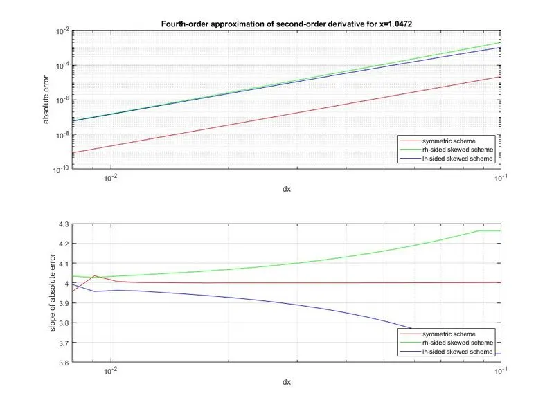
As we can see from the plot, the three schemes approximate the second-order derivative with almost the same drop rate (approximately 4).
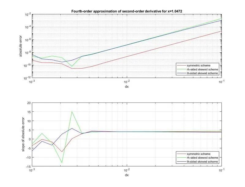
However, if we continue to decrease the dx interval, strange behaviours appear, maybe due to computational errors, even though the approximation continues to be good (below to `10^(-8)`). If we continued to decrease dx, the plot would be even more chaotic.
Why do we need skewed schemes rather than symmetric schemes?
Skewed schemes might be useful:
- at the boundary of the domain, where there are points available only on the right side or only on the left side
- when we know how the information "flows" inside the domain. To use the right scheme can determine the stability of the solution. The method of characteristics of PDEs has the purpose to choose the correct schemes to use into our simulation in order to make it stable.
%
%  File    :   main.m
%
%  Author  :   Matteo Agositnone
%  Date    :   07.02.2021
%
%  Course  :   SKILL-LYNC - Introduction to CFD using MATLAB and OpenFOAM
%
%  Challenge   : Week 3 - Taylor table method and Matlab code
%  Description :
%  Derive the 4th-order approximation of the 2nd-order derivative, using a
%  central scheme, a right-sided skewed scheme, and a left-sided skewed
%  scheme. Compare the absolute error in a plot with respect to the second
%  derivative of the function
%             f(x) = exp(x).*cos(x)
%  at a desired point x, using a desired set of intervals

clearvars
close all
clc

%% STEP 1: DEFINE DATA

Q = 2;          % Derivative order
P = 4;          % Accuracy order

% Number of points in the stencil for a symmetric scheme (HINT i)
N_sym = Q + P - 1;
% Number of points in the stencil for a skewed scheme (HINT ii)
N_skw = Q + P;

% Define a probe point x
x = pi/3;

% Define a set of intervals dx
dx = logspace(-2.2,-1,20);

%% STEP 2: FIND TAYLOR TABLE COEFFICIENTS FOR A SYMMETRIC SCHEME

% The left-side coefficient of the stencil (that multiplies dx) has value:
left_sym = -(N_sym - 1)/2;

% Let's create an empty Taylor table...
taylor_table_sym = zeros(N_sym);

% The following loop fills the Taylor table for a central scheme

for i = 1 : N_sym
    for j = 1 : N_sym

        % The value to pass first is the most left point in the stencil
        taylor_table_sym(i,j) = taylor_expansion_coefficient(left_sym + i - 1, j - 1);

    end
end

% Now we need to solve the system of equations AX = B. Let's define B:
B = zeros(N_sym,1);

% we want set to 1 only the row corresponding to the order derivative we
% want to find
B(Q + 1) = 1;

% We take the reciprocal of the Taylor table
A = taylor_table_sym';

% We finally find the coefficients!
X = A\B;

%% STEP 3: FIND TAYLOR TABLE COEFFICIENTS FOR A RIGHT-SIDED SKEWED SCHEME

% The left-side coefficient of the stencil (that multiplies dx) has value:
left_rh_skw = 0;

% Let's create an empty Taylor table...
taylor_table_rh_skw = zeros(N_skw);

% The following loop fills the Taylor table for a central scheme

for i = 1 : N_skw
    for j = 1 : N_skw

        % The value to pass first is the most left point in the stencil
        taylor_table_rh_skw(i,j) = taylor_expansion_coefficient(left_rh_skw + i - 1, j - 1);

    end
end

% Now we need to solve the system of equations CY = D. Let's define D:
D = zeros(N_skw,1);

% we want set to 1 only the row corresponding to the order derivative we
% want to find
D(Q + 1) = 1;

% We take the reciprocal of the Taylor table
C = taylor_table_rh_skw';

% We finally find the coefficients!
Y = C\D;

%% STEP 4: FIND TAYLOR TABLE COEFFICIENTS FOR A LEFT-SIDED SKEWED SCHEME

% The left-side coefficient of the stencil (that multiplies dx) has value:
left_lh_skw = -(N_skw - 1);

% Let's create an empty Taylor table...
taylor_table_lh_skw = zeros(N_skw);

% The following loop fills the Taylor table for a central scheme

for i = 1 : N_skw
    for j = 1 : N_skw

        % The value to pass first is the most left point in the stencil
        taylor_table_lh_skw(i,j) = taylor_expansion_coefficient(left_lh_skw + i - 1, j - 1);

    end
end

% Now we need to solve the system of equations EZ = F. Let's define F:
F = zeros(N_skw,1);

% we want set to 1 only the row corresponding to the order derivative we want to find
F(Q + 1) = 1;

% We take the reciprocal of the Taylor table
E = taylor_table_lh_skw';

% We finally find the coefficients!
Z = E\F;

%% STEP 5: Comparison with the analytical second derivative
%       f(x) = exp(x).*cos(x)
%       f''(x) = -2*exp(x).*sin(x)

% the analytical second-order derivative is:
d2f_dx2 = -2.*exp(x).*sin(x);

% Calculate the x and y values of the stencil for each interval dx

% SYMMETRIC SCHEME
stencil_sym_x = zeros(N_sym,length(dx));

for i = 1 : N_sym

    stencil_sym_x(i,:) = x + (left_sym + i - 1).*dx;

end

stencil_sym_y = f(stencil_sym_x);

% the fourth-order approximation of the second-order derivative is:
d2f_dx2_sym = (X' * stencil_sym_y)./(dx).^2;

% absolute error of a symmetric scheme:
abs_err_sym = abs(d2f_dx2 - d2f_dx2_sym);

% RIGHT-SIDED SKEWED SCHEME
stencil_rh_skw_x = zeros(N_skw,length(dx));

for i = 1 : N_skw

    stencil_rh_skw_x(i,:) = x + (left_rh_skw + i - 1).*dx;

end

stencil_rh_skw_y = f(stencil_rh_skw_x);

% the fourth-order approximation of the second-order derivative is:
d2f_dx2_rh_skw = (Y' * stencil_rh_skw_y)./(dx).^2;

% absolute error of a rh-sided skewed scheme:
abs_err_rh_skw = abs(d2f_dx2 - d2f_dx2_rh_skw);

% LEFT-SIDED SKEWED SCHEME
stencil_lh_skw_x = zeros(N_skw,length(dx));

for i = 1 : N_skw

    stencil_lh_skw_x(i,:) = x + (left_lh_skw + i - 1).*dx;

end

stencil_lh_skw_y = f(stencil_lh_skw_x);

% the fourth-order approximation of the second-order derivative is:
d2f_dx2_lh_skw = (Z' * stencil_lh_skw_y)./(dx).^2;

% absolute error of a rh-sided skewed scheme:
abs_err_lh_skw = abs(d2f_dx2 - d2f_dx2_lh_skw);

%% STEP 6: PLOT RESULTS
subplot(2,1,1)
loglog(dx,abs_err_sym,'r')
title(strcat('Fourth-order approximation of second-order derivative for x= ',num2str(x)))
xlabel('dx')
ylabel('absolute error')
grid on
hold on
loglog(dx,abs_err_rh_skw,'g')
loglog(dx,abs_err_lh_skw,'b')
legend('symmetric scheme','rh-sided skewed scheme','lh-sided skewed scheme','Location','southeast')

subplot(2,1,2)
semilogx(dx,logSlope(abs_err_sym,dx),'r')
xlabel('dx')
ylabel('slope of absolute error')
grid on
hold on
semilogx(dx,logSlope(abs_err_rh_skw,dx),'g')
semilogx(dx,logSlope(abs_err_lh_skw,dx),'b')
legend('symmetric scheme','rh-sided skewed scheme','lh-sided skewed scheme','Location','southeast')
%
%  Function:   f.m
%
%  Author  :   Matteo Agositnone
%  Date    :   07.02.2021
%
%  Course  :   SKILL-LYNC - Introduction to CFD using MATLAB and OpenFOAM
%
%  Challenge   : Week 3 - Taylor table method and Matlab code
%  Description : The function takes a vector as input, and returns the
%                assigned function f(x)

function y = f(x)

y = exp(x).*cos(x);

end
%
% Function: taylor_expansion_coefficient.m
%
% Author : Matteo Agositnone
% Date : 07.02.2021
%
% Course : SKILL-LYNC - Introduction to CFD using MATLAB and OpenFOAM
%
% Challenge : Week 3 - Taylor table method and Matlab code
% Description : The function calculates the coefficient of the Taylor
% expansion, given as input the multiple of the interval
% Delta x, and the order of the derivative
function coeff = taylor_expansion_coefficient(delta_x_multiplier, order_of_derivative)
coeff = (delta_x_multiplier^order_of_derivative)/factorial(order_of_derivative);
end
%
%  Function:   logSlope.m
%
%  Author  :   Matteo Agositnone
%  Date    :   07.02.2021
%
%  Course  :   SKILL-LYNC - Introduction to CFD using MATLAB and OpenFOAM
%
%  Challenge   : Week 3 - Taylor table method and Matlab code
%  Description : The function takes two vectors as input, and returns a
%                vector that contains the point-to-point slope of the
%                loglog chart.


function output = logSlope(input,dx)
% The output vector has  in theory one value less that the input vector, since it is
% evaluating intervals between points. However, in order to avoid further
% complications on plotting graphs, I assumed the output vactor is of the same
% size of the input vector, and that the penultimate and the
% ultimate values are coincident

output = zeros(length(input),1);

% Find the slope of all the points except the last point...
for i = 1:length(input)-1

    output(i) = (log(input(i+1)/input(i)))/log((dx(i+1)/dx(i)));

end

% ...which we assume to be equal to the penultimate value
output(end) = output(end - 1);

end