Week 5.1 - Mid term project - Solving the steady and unsteady 2D heat conduction problem
Objective:- 1. Steady state analysis & Transient State Analysis
Solve the 2D heat conduction equation by using the point iterative techniques that were taught in the class. The Boundary conditions for the problem are as follows;
Top Boundary = 600 K
Bottom Boundary = 900 K
Left Boundary = 400 K
Right Boundary = 800 K
You will implement the following methods for solving implicit equations.
- Jacobi
- Gauss-seidel
- Successive over-relaxation
Your absolute error criteria is 1e-4
Solution:-
Steady State 2D Heat conduction equation
Steady state is defined when all the fluid properties does not change with respect to time
Below is the 2D heat conduction equation
`(delT)/(delt) + alpha * [(del^2T)/(delx^2) + (del^2T)/(dely^2)] = 0`
For steady state the time derivative is equal to zero
Therefore the equation reduces to
`[(del^2T)/(delx^2) + (del^2T)/(dely^2)] = 0`
Discretization for Steady State
`(T_L – 2*T_P + T_R)/(Deltax^2) + (T_T – 2*T_P + T_B)/(Deltay^2) = 0`
Where `T_L = T_(i-1,j)`
`T_R = T_(i+1,j)`
`T_T = T_(i,j-1)`
`T_B = T_(i,j+1)`
`T_P*[(2*(Deltax^2 + Deltay^2))/(Deltax^2*Deltay^2)] = (T_L + T_R)/(Deltax^2) + (T_T + T_B)/(Deltay^2)`
Therefore, `T_P = K_1 * (T_L + T_R) + K_2*(T_T + T_B)`
Where, `K_1 = (Deltay^2)/(2*(Deltax^2+Deltay^2))`
`K_2 = (Deltax^2)/(2*(Deltax^2+Deltay^2))`
Solving the above equation through 3 different iterative techniques
- Jacobi method
`(T_P)^(n+1) = K_1 * (T_L + T_R)^n + K_2*(T_T + T_B)^n`
- Gauss seidel
`T_P^(n+1) = K_1 * (T_L + T_R)^(n+1) + K_2*(T_T + T_B)^(n+1)`
- SOR
`T_P^(n+1) = T_P^n*(1-omega) + omega*(K_1 * (T_L + T_R)^(n+1) + K_2*(T_T + T_B)^(n+1))`
Transient State Heat Conduction
Here the fluid properties will change with respect to time
Formula for Transient Heat Conduction
`(delT)/(delt) + alpha * [(del^2T)/(delx^2) + (del^2T)/(dely^2)] = 0`
Discretization for Unsteady State
`(T_P^(n+1) – T_P^n)/(Deltat) - alpha*((T_L – 2*T_P + T_R)/(Deltax^2) + (T_T – 2*T_P + T_B)/(Deltay^2)) = 0`
If the above equation is calculated for `n^(th)` time step then the solution is called as explicit solution and if it is calculated for `(n+1)^(th)` time step then the solution is called implicit solution
Formula for Explicit method
`T_P^(n+1) = T_P^n + K_1*(T_L – 2*T_P + T_R)^n + K_2*(T_T – 2*T_P + T_B)^n`
Where, `K_1 = (alpha*Deltat)/(Deltax^2)`
`K_2 = (alpha*Deltat)/(Deltay^2)`
`K_1` and `K_2` are also known as CFL number
For explicit diffusion problems
`CFL <= 0.5`
`CFL_x + CFL_y <= 0.5`
Formula for Implicit Method
- Jacobi method
`T_P^(n+1) = 1/(1+2*K_1+2*K_2) * [T_P^n + K_1*(T_L^n + T_R^n) + K_2*(T_T^n + T_B^n)]`
- Gauss seidel method
`T_P^(n+1) = 1/(1+2*K_1+2*K_2) * [T_P^n + K_1*(T_L^(n+1) + T_R^n) + K_2*(T_T^(n+1) + T_B^n)]`
- SOR method
`T_P^(n+1) = T_P^n*(1-omega) + omega*(1/(1+2*K_1+2*K_2) * [T_P^n + K_1*(T_L^(n+1) + T_R^n) + K_2*(T_T^(n+1) + T_B^n)])`
Matlab Program for Explicit Steady State Heat Conduction
l = 1;
nx = 10;
ny = 10;
dx = l/(nx-1);
dy = l/(ny-1);
K = 2*((dx^2 + dy^2)/(dx^2*dy^2));
x = linspace(0,1,nx);
y = linspace(0,1,ny);
T = ones(nx,ny);
T([2:9],[2:9]) = 300;
T([1:1],[2:9]) = 600;
T([10:10],[2:9]) = 900;
T([2:9],[1:1]) = 400;
T([2:9],[10:10]) = 800;
T(1,1) = (T(1,2)+T(2,1))/2;
T(1,end) = (T(1,9)+T(2,10))/2;
T(end,1) = (T(9,1)+T(10,2))/2;
T(end,end) = (T(9,10)+T(10,9))/2;

T_initial = T;
T_old = T;

[xx,yy] = meshgrid(x,y);
tol = 1e-4;
error = 9e9;
w = 1.5;

Iterative_solver = input('Enter 1 for Jacobi, 2 for Gauss Siedel and 3 for SOR = ')

if Iterative_solver == 1
    jacobi_iter = 1;
    while(error > tol)
        for i = 2:nx-1
            for j = 2:ny-1
                term1 = ((1/K)*((T_old(i-1,j)+T_old(i+1,j))/dx^2));
                term2 = ((1/K)*((T_old(i,j-1)+T_old(i,j+1))/dy^2));
                T(i,j) = term1 + term2;
            end
        end
        error = max(max(abs(T_old-T)))
        T_old = T;
        jacobi_iter = jacobi_iter + 1
     [C,h] = contourf(xx,yy,T);
colorbar;
colormap(jet)
clabel(C,h)
pause(0.03)
title(sprintf('Steady State Heat conduction using Jacobi method n Number of iterations: %d',jacobi_iter))
    end

end

if Iterative_solver == 2
    gauss_siedel_iter = 1;
    while(error > tol)
        for i = 2:nx-1
            for j = 2:ny-1
                term1 = ((1/K)*((T(i-1,j)+T_old(i+1,j))/dx^2));
                term2 = ((1/K)*((T(i,j-1)+T_old(i,j+1))/dy^2));
                T(i,j) = term1 + term2;
            end
        end
        error = max(max(abs(T_old-T)));
        T_old = T;
        gauss_siedel_iter = gauss_siedel_iter + 1

        [C,h] = contourf(xx,yy,T);
    colorbar;
colormap(jet)
clabel(C,h)
pause(0.03)
title(sprintf('Steady State Heat conduction using Gauss siedel method n Number of iterations: %d',gauss_siedel_iter))
    end

end

if Iterative_solver == 3
    SOR_iter = 1;
    while(error > tol)
        for i = 2:nx-1
            for j = 2:ny-1
                term1 = ((1/K)*((T(i-1,j)+T_old(i+1,j))/dx^2));
                term2 = ((1/K)*((T(i,j-1)+T_old(i,j+1))/dy^2));
                T(i,j) = (1-w)*T_old(i,j) + w*(term1 + term2);
            end
        end
        error = max(max(abs(T_old-T)));
        T_old = T;
        SOR_iter = SOR_iter + 1

        [C,h] = contourf(xx,yy,T);
    colorbar;
colormap(jet)
clabel(C,h)
pause(0.03)
title(sprintf('Steady State Heat conduction using SOR method n Number of iterations: %d',SOR_iter))
    end

end
Result:-
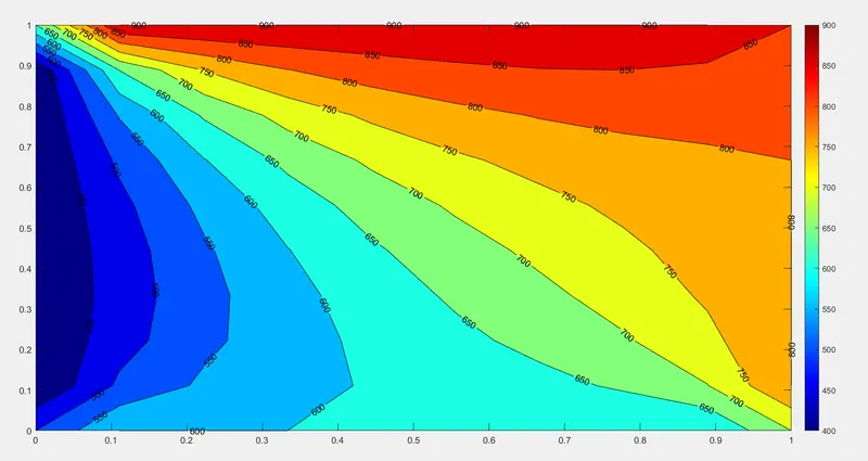
Jacobi method
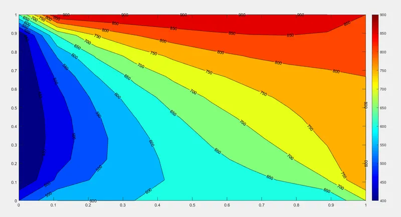
Gauss seidel method
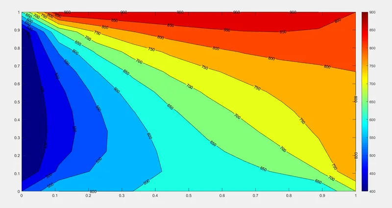
SOR method
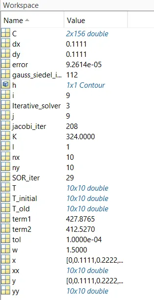
In the workspace above it can be seen that SOR method uses minimum iteration and converges faster than Jacobi and Gauss seidel method
The number of iterations for the above three methods are as follows
Jacobi = 208
Gauss siedel = 112
SOR = 29
The number of iterations required by SOR method to converge depends on the value of `omega` i.e relaxation factor
The number of iterations changes as we change the value of `omega`
Matlab Program for Unsteady State Explicit Method
l = 1;
nx = 10;
ny = 10;
nt = 100;
x = linspace(0,1,nx);
y = linspace(0,1,ny);
dx = x(2)-x(1);
dy = y(2)-y(1);
dt = 0.001;
alpha = 1.4;
k_1 = (alpha*dt)/(dx^2);
k_2 = (alpha*dt)/(dy^2);
CFL = k_1+k_2
T = ones(nx,ny);
T([2:end-1],[2:end-1]) = 300;
T([1:1],[2:end-1]) = 600;
T([end:end],[2:end-1]) = 900;
T([2:end-1],[1:1]) = 400;
T([2:9],[end:end]) = 800;
T(1,1) = (T(1,2)+T(2,1))/2;
T(1,end) = (T(1,9)+T(2,10))/2;
T(end,1) = (T(9,1)+T(10,2))/2;
T(end,end) = (T(9,10)+T(10,9))/2;

T_old = T;
T_initial = T_old;

[xx,yy] = meshgrid(x,y);

error = 9e9;
tol = 1e-4;
explicit_iter = 0;

    for m = 1:nt

        for i = 2:nx-1
            for j = 2:ny-1
               term1 = T_old(i,j);
               term2 = k_1*(T_old(i-1,j) - (2*T_old(i,j)) + T_old(i+1,j));
               term3 = k_2*(T_old(i,j-1) - (2*T_old(i,j)) + T_old(i,j+1));
               T(i,j) = term1 + term2 + term3;
            end
        end
        T_old = T;
        explicit_iter = explicit_iter + 1;
        [C,h] = contourf(xx,yy,T);
colorbar;
colormap(jet)
clabel(C,h)
pause(0.03)
title(sprintf('Unsteady State Heat conduction using Explicit method n Number of iterations: %d',explicit_iter))
    end
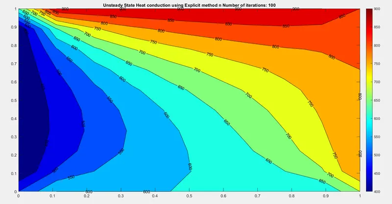
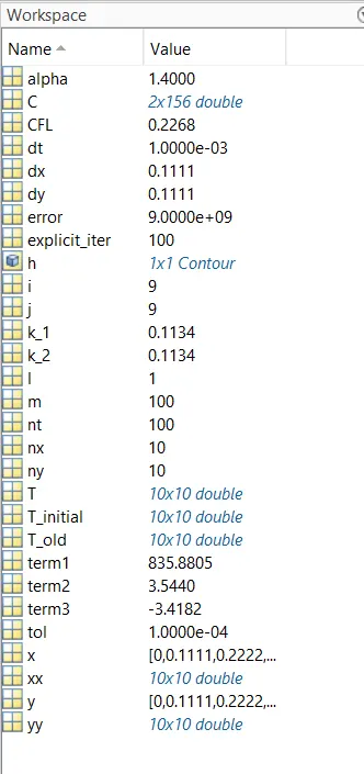
Result:-
Matlab Program for Unsteady State Implicit Method
l = 1;
nx = 10;
ny = 10;
nt = 100;
x = linspace(0,1,nx);
y = linspace(0,1,ny);
dx = x(2)-x(1);
dy = y(2)-y(1);
dt = 0.001
alpha = 1.5
k_1 = (alpha*dt)/dx^2
k_2 = (alpha*dt)/dy^2
CFL = k_1+k_2

T = ones(nx,ny);
T([2:9],[2:9]) = 300;
T([1:1],[2:9]) = 600;
T([10:10],[2:9]) = 900;
T([2:9],[1:1]) = 400;
T([2:9],[10:10]) = 800;
T(1,1) = (T(1,2)+T(2,1))/2;
T(1,end) = (T(1,9)+T(2,10))/2;
T(end,1) = (T(9,1)+T(10,2))/2;
T(end,end) = (T(9,10)+T(10,9))/2;

T_old = T;
T_initial = T_old;

[xx,yy] = meshgrid(x,y);
tol = 1e-4;
error = 9e9;
w = 1.1;
term1 = 1/(1+2*k_1+2*k_2);
term2 = k_1*term1;
term3 = k_2*term1;

Iterative_solver = input('Enter 1 for Jacobi, 2 for Gauss Siedel and 3 for SOR = ')

if Iterative_solver == 1
    jacobi_iter = 0;
    for m = 1:nt
        error = 20;
    while(error > tol)
        for i = 2:nx-1
            for j = 2:ny-1
                H = T_old(i-1,j) + T_old(i+1,j);
                V = T_old(i,j-1) + T_old(i,j+1);
                T(i,j) = (term1*T_initial(i,j)) + (term2*H) + (term3*V);
            end
        end
        error = max(max(abs((T_old-T))));
        T_old = T;
        jacobi_iter = jacobi_iter + 1;
    end

    T_initial = T;
    pause(0.03)
 [C,h] = contourf(xx,yy,T);
colorbar;
colormap(jet)
clabel(C,h)
title(sprintf('Unsteady State Heat conduction using Jacobi method n Number of iterations: %d',jacobi_iter))
    end

end


if Iterative_solver == 2
     gauss_siedel_iter = 1;
    for m = 1:nt
   error = 2;
    while(error > tol)
        for i = 2:nx-1
            for j = 2:ny-1

                H = T(i-1,j) + T_old(i+1,j);
                V = T(i,j-1) + T_old(i,j+1);
                T(i,j) = (term1*T_initial(i,j)) + (term2*H) + (term3*V);
            end
        end
        error = max(max(abs(T_old-T)));
        T_old = T;
        gauss_siedel_iter = gauss_siedel_iter + 1;
    end
T_initial = T;

[C,h] = contourf(xx,yy,T);
colorbar;
colormap(jet)
clabel(C,h)
pause(0.03)
title(sprintf('Unsteady State Heat conduction using Gauss siedel method n Number of iterations: %d',gauss_siedel_iter))
    end

end


if Iterative_solver == 3
    SOR_iter = 0;
    for m = 1:nt
    error = 1;
    while(error > tol)
        for i = 2:nx-1
            for j = 2:ny-1

                H = T_old(i-1,j) + T_old(i+1,j);
                V = T_old(i,j-1) + T_old(i,j+1);
                T(i,j) = ((1-w)*(T_old(i,j))) + (w*(term1*T_initial(i,j) + (term2*H) + (term3*V)));
            end
        end
        error = max(max(abs((T_old-T))));
        T_old = T;
        SOR_iter = SOR_iter + 1;
    end

    T_initial = T;
    [C,h] = contourf(xx,yy,T);
colorbar;
colormap(jet)
clabel(C,h)
pause(0.03)
title(sprintf('Unsteady State Heat conduction using Jacobi method n Number of iterations: %d',SOR_iter))

    end

end
Result:-
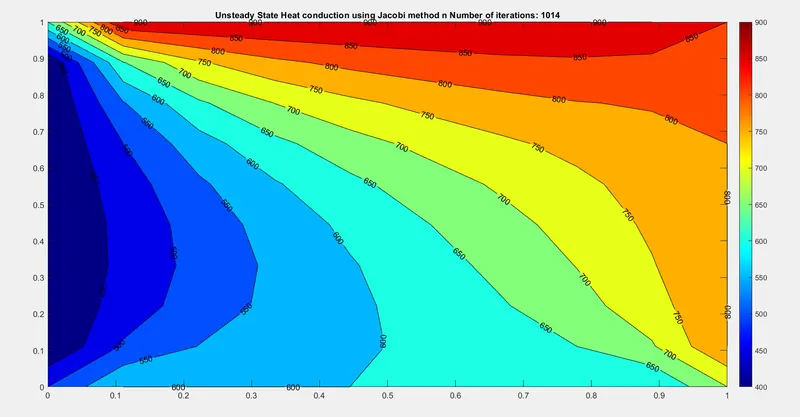
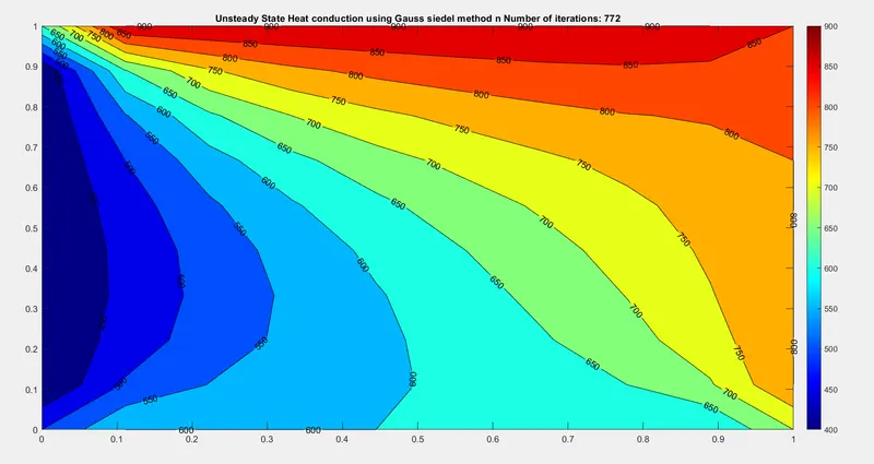
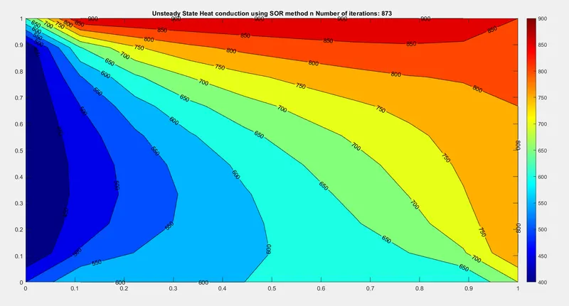
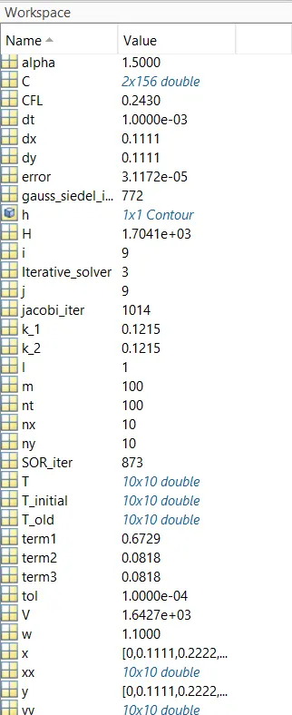
In the workspace above it can be seen that Gauss seidel method uses minimum iteration and converges faster than Jacobi and SOR method
The number of iterations for the above three methods are as follows
Jacobi = 1014
Gauss siedel = 772
SOR = 873
The number of iterations required by SOR method to converge depends on the value of `omega` i.e relaxation factor
The number of iterations changes as we change the value of `omega`
We can see that the explicit method gives faster result as compared to implicit method. This is because it does not require guess vlaues and iterations for convergence as it depend only on the previous values which had already been calculated