Week 5.1 - Mid term project - Solving the steady and unsteady 2D heat conduction problem
OBJECTIVE:
1. Steady state analysis & Transient State Analysis
Solve the 2D heat conduction equation by using the point iterative techniques that were taught in the class. The Boundary conditions for the problem are as follows;
Top Boundary = 600 K
Bottom Boundary = 900 K
Left Boundary = 400 K
Right Boundary = 800 K
You will implement the following methods for solving implicit equations.
1. Jacobi
2. Gauss-seidel
3. Successive over-relaxation
Your absolute error criteria is 1e-4
Make sure to use "INSERT CODE SAMPLE" option to paste the code here. Post screenshots of the plots and use the projects.skill-lync.com page to Publish your findings.
2. You will write code for both implicit and explicit schemes (This is for the Transient Analysis only)
THEORY:
Introduction:
Explicit Method: When a direct computation is made for an unknown quality in terms of known quantity. This computation is called Explicit. This method requires stability criteria which when satisfied leads to stable solution. Because of the stability criteria small time steps has to be taken to obtain stable solutions. With decrease in time step the number of computations increases and hence the computational time required for the solution to converge is less and accuracy of the solution is high.
Implicit Method: When a computation is made for dependent variable are defined by set of equations and a matrix is involved to find the unknown variable. This computation is called Implicit method. This method is unconditionally stable as a result, no stability criteria is required to obtain a stable results and the computational time required for the solution to converge is high and accuracy of the solution is less relative to explicit method because this method uses simultaneous equations and uses guess values as the initial values to find the approximated values. If the guess values are closer to the desired value the computation time is less. As there is no stability criteria requirement larger time steps can be used.
In order to solve for dependent variable iterative solvers are used. Iterative solvers used are:
- Jacobi iterative solver (Jacobi Method)
- Gauss seidel iterative solver (Gauss seidel Method)
- Successive over relaxation iterative solver (SOR Method)
Iterative solvers:
Jacobi iterative solver: In this method the temperature at n+1th iteration is found using old values of the temperature defined at nth iterations. Using the approximation obtained iterations procedure it continued until the desired accuracy of the solution is obtained.
Gauss seidel iterative solver: In this type iterative solver, temperature at n+1 iteration uses values of n+1 iteration that have already been computed. By this way old approximated values are overwritten with new approximate values for the iterations performed. Unlike Jacobi, Gauss seidel require one storage vector which can be overwritten with each computation. This helps for the solution to converge faster than the Jacobi method.
Successive over relaxation iterative solver: In this type of iterative solver relaxation factor is used which helps in increasing the convergence rate. It goes by the formula:
`T^(n+1)=T^n (1-ω)+ωT(GS) or T(JACOBI)`
In the above Equation, we have:
`T(GS) or T(JACOBI)`: is the temperature value for n+1 th iteration using GAUSS SEIDAL METHOD or JACOBI METHOD.
`ω`:is the relaxation factor.
Range of `ω`is between 0<`ω`<2. Now, when `ω`>1: OVER RELAXATION. Again, when `ω`<1: UNDER RELAXATION.
OVER RELAXATION STATE(`ω`>1): This condition is used when the temperature gradient is low and due to this condition larger time steps are used to obtain the steady state i.e.,for the values to converge at faster rate.
UNDER RELAXATION STATE(`ω`<1): This condition is used when the temperature gradient is high and due to this condition the time step does not over shoot and helps to converge at a faster rate.
2-DIMENSIONAL HEAT CONDUCTION EQUATION: The heat equation is a second order partial differential equation that describes how the distribution of some quantity (such as heat) evolves over time in a solid medium, as it spontaneously flows from places where it is higher towards where it is lower.
Heat transfer is the transfer of thermal energy from a body, at a high temperature, to another at a lower temperature . This transfer of thermal energy may occur under steady or unsteady state conditions.
In this project, we will be computing the 2D heat conduction problem. But in reality, there is no such thing as 2 dimensional heat conduction, there is only 3D heat conduct ion. The 2D heat conduction analysis is generally done to observe the flow and its properties in 2D.
The, 2D Heat conduction Equation is: `(∂T)/(∂t)=∝((∂^2 T)/(∂x^2 )+(∂^2 T)/(∂y^2 ))` .....(1)
In the above Equation we have `(∂T)/(∂t)` as the Time derivative, `((∂^2 T)/(∂x^2 )+(∂^2 T)/(∂y^2 ))` as the spatial derivative and `∝` as the thermal diffusivity.
Equation..(1) is hyperbolic in nature which can be discretized using forward differencing scheme and the spacial derivatives are elliptical in nature which can be discretized using central differencing scheme.
STEADY STATE ANALYSIS:
Steady state analysis occures when `(∂T)/(∂t)`=0.Hence, from Equation..(1) we get `(∂^2 T)/(∂x^2 )+(∂^2 T)/(∂y^2 )=0`
DISCRITIZATION OF STEADY STATE EQUATION:
We use CENTRAL DIFFERENCING SCHEME(CDS) to discritize the steady state equation,hence we have:
`(T_L-2T_P+T_R)/((∆x)^2) +(T_T-2T_P+T_B)/((∆y)^2) =0`
In the above Equation we have: `T_P=T_i,j`, `T_L=T_(i-1,j)`, `T_R=T_(i+1,j)`, `T_T=T_(i,j-1)`, `T_B=T_(i,j+1)`
Now, solving for T(i,j) we get: `T_P=K_1(T_L+T_R)+K_2(T_T+T_B)`, where `K_1=(∆y)^2/(2{(∆x)^2+(∆y)^2})` & `K_2=(∆x)^2/(2{(∆x)^2+(∆y)^2})`
Now, we solve the 2-dimensional Heat Conduction Equation through the iterative techniques, we get:
JACOBI METHOD OF SOLVING:
`(T_P)^(n+1)=K_1(T_L+T_R)^n+K_2(T_T+T_B)^n`
Here, n represents the generation of the value that is beingcalculated as this is an iterative method.
GAUSS SEIDEL METHOD OF SOLVING:
`(T_P)^(n+1)=K_1(T_L+T_R)^n+K_2(T_T+T_B)^n`
The GAUSS-SEIDEL METHOD is similar to the JACOBI METHOD with only one difference. In this method, we use the previously calculated value for the next generation of that value.
SUCCESSIVE OVER-RELAXATION (SOR) METHOD OF SOLVING:
`(T_P)^(n+1)= (T_P)^n(1-ω) +ω[K_1(T_L+T_R)^(n+1)+K_2(T_T+T_B)^(n+1)]`
The SUCCESSIVE OVER-RELAXATION (SOR) METHOD is the variant of the Gauss Seidel Method for solving a linear system of equation.
TRANSIENT STATE ANALYSIS:
A Fluid state in which there is a change in the fluid property with respect to time is known as an Unsteady or a Transient State. Transient State conditions are a precursor to steady state conditions. No system exists initially under steady state conditions. Sometime must pass, after heat transfer is initiated, before the system reaches steady state. During that period of transition the system is under Transient State conditions.
The formula for transient state is: `(∂T)/(∂t)=∝((∂^2 T)/(∂x^2 )+(∂^2 T)/(∂y^2 ))`
DISCRITIZATION OF TRANSIENT STATE EQUATION:
We use CENTRAL DIFFERENCING SCHEME(CDS) to discritize the steady state equation,hence we have:
`(T_P^(n+1)-T_P^n)/((∆t))-α[(T_L-2T_P+T_R)/((∆x)^2) +(T_T-2T_P+T_B)/((∆y)^2) ]=0`
In the above Equation we have: `T_P=T_i,j`, `T_L=T_(i-1,j)`, `T_R=T_(i+1,j)`, `T_T=T_(i,j-1)`, `T_B=T_(i,j+1)`
Now, solving for T(i,j) we get: `(T_P)^(n+1)=(T_P)^n(1-2k_1-2k_2)+K_1(T_L+T_R)^n+K_2(T_T+T_B)^n`
where `K_1=α(∆t)/(∆x)^2` & `K_2=α(∆t)/(∆y)^2`
Stability criteria: `K_1+K_2 ≤ 0.5` {FOR EXPLICIT SCHEME}
Solving the Transient Heat Conduction Equation using the same three iterative methods which are used in steady state condition by implementing them in both implicit and explicit forms.
IMPLICIT SCHEME OF TRANSIENT STATE EQUATION:
JACOBI METHOD OF SOLVING:
In the implicit form, the Transient Equation is represented as:
`(T_P)^(n+1)=(T_P)^n+K_1(T_L^(n+1)-2T_P^(n+1)+T_R^(n+1))+K_2(T_T^(n+1)-2T_P^(n+1)+T_B^(n+1))`
The, above Equation can be simplified to after arranging n+1 term:
`(T_P)^(n+1)={(T_P)^n+K_1(T_L^(n+1)+ T_R^(n+1))+K_2(T_T^(n+1) +T_B^(n+1))}/{1+2k_1+2k_2}`
Hence, the implicit form of JACOBI METHOD for transient heat conduction equation:
`(T_P)^(n+1)={(T_P)^n+K_1(T_L^(n)+ T_R^(n))+K_2(T_T^(n) +T_B^(n))}/{1+2k_1+2k_2}`
GAUSS-SEIDEL METHOD OF SOLVING:
`(T_P)^(n+1)={(T_P)^n+K_1(T_L^(n+1)+ T_R^(n))+K_2(T_T^(n) +T_B^(n+1))}/{1+2k_1+2k_2}`
SUCCESSIVE OVER-RELAXATION (SOR) METHOD OF SOLVING:
`(T_P)^(n+1)= (T_P^n)(1-ω) +ω{{(T_P)^n+K_1(T_L^(n+1)+ T_R^(n))+K_2(T_T^(n) +T_B^(n+1))}/{1+2k_1+2k_2}}`
EXPLICIT SCHEME OF TRANSIENT STATE EQUATION:
In the case of explicit functions,we arrange the n terms and simplify to obtain:
JACOBI METHOD OF SOLVING:
`T_P^(n+1)=T_P^n(1-2K_1-2K_2)+K_1(T_L^n+T_R^n)+K_2(T_T^n+T_B^n)`
GAUSS-SEIDEL METHOD OF SOLVING:
`T_P^(n+1)=T_P^n(1-2K_1-2K_2)+K_1(T_L^(n+1)+T_R^n)+K_2(T_T^n+T_B^(n+1))`
SUCCESSIVE OVER-RELAXATION (SOR) METHOD OF SOLVING:
`T_P^(n+1)= T_P^n (1-ω) +ω{T_P^n(1-2K_1-2K_2)+K_1(T_L^(n+1)+T_R^n)+K_2(T_T^n+T_B^(n+1))}`
MATLAB CODE FOR STEADY STATE ANALYSIS:
clear all
close all
clc


%initial conditions
L=1; %length of the domain
nx=input ('For the uniformly space grid please enter the number of grid points:');
ny=nx;


x=linspace (0,L,nx);
y=linspace (L,0,ny);
dx=L/(nx-1); %providing the spacing between the grid points along x axis
dy=L/(ny-1); %providing the spacing between the grid points along y axis
error=9e9;
tol=1e-4;

%Defining Bound ary Conditions

T_L=400;
T_R=800;
T_T=600;
T_B=900;

%Temperature Matrix
T=298*ones(nx,ny);
T(1,:)=T_B;
T(end, :)=T_T;
T(:,1)=T_L;
T(:,end)=T_R;


%Edge Refining
T(1,1)= (900+400)/2;
T(1,end)=(900+800)/2;
T(end,1)=(400+600)/2;
T(end,end)=(800+600)/2;


%Calculation of relaxation factor
%omega=2/(l+sin(pi*dx));
omega=1.2;


%Creating a copy of old values
[X,Y]=meshgrid (x,y);
Told =T;


iterative_solver=input(' l)Jacobi 2)Gauss Seidel 3)SOR and Enter an option for the type of solver you would like to use:');

k=2/(dx^2) + 2/(dy^2);

tic
if iterative_solver==1
    jacobi_iter=1;
    while(error>tol)
        for i=2:nx-1
            for j=2 :ny-1
                term1= (Told (i-1,j)+Told (i+1,j))/(k*(dx^2));
                term2=(Told (i,j-1)+Told (i,j+1))/(k*(dy^2));
                T(i,j)=term1+term2;
            end
        end
        error=max(max (abs(Told-T)));
        Told=T;
        jacobi_iter=jacobi_iter+1;
    end

    figure(1)
    [A,B]=contourf(X,Y,T);
    set(gca,'YDIR','reverse')
    colorbar
    colormap(jet)
    clabel(A,B);
    text=sprintf('Jacobi Iterations = %d',jacobi_iter);
    ylabel('Y ')
    title(text)
    pause (0.03)
end


if iterative_solver==2
    gs_iter=1;
    while(error>tol)
        for i=2:nx-1
            for j=2 :ny-1
                terml= (T(i-1,j)+Told(i+1,j))/(k*(dx^2));
                term2=(T(i,j-1)+Told(i,j+1))/(k*(dy^2));
                T(i,j)=terml+term2;
            end
        end
        error=max (max (abs(Told-T)));
        Told=T;
        gs_iter=gs_iter+1;
    end
    figure(1)
    [A,B ]=contourf(X,Y,T);
    set(gca,'YDIR','reverse')
    colorbar
    colormap(jet)
    clabel(A,B);
    text=sprintf('Gauss Seidel Iterations = %d ',gs_iter);
    ylabel('Y ')
    title(text)
    pause (0.03)
end

if iterative_solver==3
    sor_iter=1;
    while(error>tol)
        for i=2:nx-1
            for j=2:ny-1
                term1=(T(i-1,j)+Told(i+1,j))/(k*(dx^2));
                term2=(T(i,j-1)+Told(i,j+1))/(k*(dy^2));
                T(i,j)=(1-omega)*Told(i,j)+omega*(term1+term2);
            end
        end
        error=max (max(abs(Told-T)));
        Told=T;
        sor_iter=sor_iter+1;
    end
    figure(1)
    [A,B]=contourf(X,Y,T);
    set(gca,'YDIR','reverse')
    colorbar
    colormap(jet)
    clabel(A,B);
    text=sprintf('SOR Iterations = %d ',sor_iter);
    title (text)
    ylabel('Y')
    pause(0.03)
end
OUTPUT:
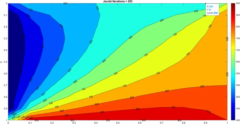
JACOBI METHOD:
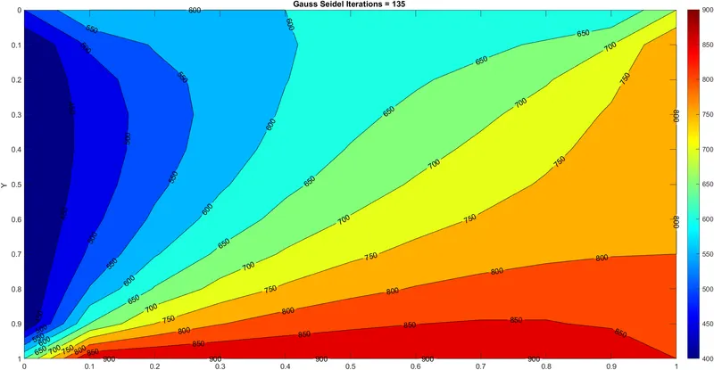
GAUSS SEIDEL METHOD:
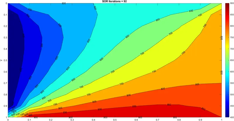
SOR METHOD:
MATLAB CODE TRANSIENT STATE ANALYSIS:
IMPLICIT SCHEME MATLAB CODE:
clear all
close all
clc


%initial conditions
L=1; %length of the domain
nx=input ('For the uniformly space grid please enter the number of grid points:');
ny=nx;


x=linspace (0,L,nx);
y=linspace (L,0,ny);
dx=L/(nx-1); %providing the spacing between the grid points along x axis
dy=L/(ny-1); %providing the spacing between the grid points along y axis
error=9e9;
tol=1e-4;
alpha=1.4;
dt=0.001;
%Defining Bound ary Conditions

T_L=400;
T_R=800;
T_T=600;
T_B=900;

%Temperature Matrix
T=298*ones(nx,ny);
T(1,:)=T_B;
T(end, :)=T_T;
T(:,1)=T_L;
T(:,end)=T_R;


%Edge Refining
T(1,1)= (900+400)/2;
T(1,end)=(900+800)/2;
T(end,1)=(400+600)/2;
T(end,end)=(800+600)/2;


k1=alpha*(dt/dx.^2);
k2=alpha*(dt/dy.^2);

CFL=k1+k2;

Told =T;
T_prev_dt=T;
iter=1;

omega=1.1;

iterative_solver=input(' l)Jacobi 2)Gauss Seidel 3)SOR and Enter an option for the type of solver you would like to use:');

tic
for nt=1:1400
    if iterative_solver==1
        term1=(1+2*k1+2*k2)^(-1);
        term2=k1*term1;
        term3=k2*term1;

        error=9e9;
        while(error>tol)
        for i=2:nx-1
            for j=2 :ny-1

                H=(Told(i-1,j)+Told(i+1,j));
                V=(Told(i,j-1)+Told(i,j+1));
                T(i,j)=(T_prev_dt(i,j)*term1)+(H*term2)+(V*term3);
            end
        end
        error=max(max(abs(Told-T)));
        Told=T;
        iter=iter+1;
        end
    end
if iterative_solver==2
    term1=(1+2*k1+2*k2)^(-1);
    term2=k1*term1;
    term3=k2*term1;

    error=9e9;
    while(error>tol)
    for i=2:nx-1
            for j=2 :ny-1

                H=(T(i-1,j)+T(i+1,j));
                V=(T(i,j-1)+T(i,j+1));
                T(i,j)=(T_prev_dt(i,j)*term1)+(H*term2)+(V*term3);

            end
    end
       error=max(max(abs(Told-T)));
       Told=T;
       iter=iter+1;
    end
end
if iterative_solver==3
    term1=(1+2*k1+2*k2)^(-1);
    term2=k1*term1;
    term3=k2*term1;

    error=9e9;
    while(error>tol)
    for i=2:nx-1
            for j=2:ny-1

                H=(T(i-1,j)+T(i+1,j));
                V=(T(i,j-1)+T(i,j+1));
                T(i,j)=(1-omega)*Told(i,j)+omega*((T_prev_dt(i,j)*term1)+(H*term2)+(V*term3));

            end
    end
       error=max(max(abs(Told-T)));
       Told=T;
       iter=iter+1;
    end
end
T_prev_dt=T;
end
Time_taken=toc;
figure(1)
    [P,Q]=contourf(x,y,T);
    set(gca,'YDIR','reverse')
    colorbar
    colormap(jet)
    clabel(P,Q);
    text=sprintf('Implicit Iteration = %d',iter);
    title (text)
    ylabel('Y')
    pause(0.03)
OUTPUT:
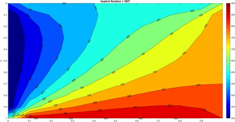
JACOBI METHOD:
GAUSS SEIDEL METHOD:
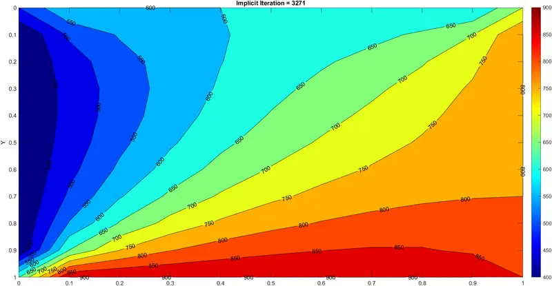
SOR METHOD:
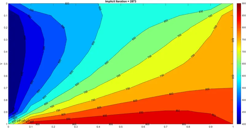
EXPLICIT SCHEME MATLAB CODE:
clear all
close all
clc


%initial conditions
L=1; %length of the domain
nx=input ('For the uniformly space grid please enter the number of grid points:');
ny=nx;


x=linspace (0,L,nx);
y=linspace (L,0,ny);
dx=L/(nx-1); %providing the spacing between the grid points along x axis
dy=L/(ny-1); %providing the spacing between the grid points along y axis
error=9e9;
tol=1e-4;
dt=0.001;
alpha=1.4;

%t=0.1;
%nt=t/dt;

%Defining Bound ary Conditions
T_L=400;
T_R=800;
T_T=600;
T_B=900;

%Temperature Matrix
T=298*ones(nx,ny);
T(1,:)=T_B;
T(end, :)=T_T;
T(:,1)=T_L;
T(:,end)=T_R;


%Edge Refining
T(1,1)= (900+400)/2;
T(1,end)=(900+800)/2;
T(end,1)=(400+600)/2;
T(end,end)=(800+600)/2;

k1=alpha*(dt/dx.^2);
k2=alpha*(dt/dy.^2);

[X,Y]=meshgrid (x,y);
Told=T;

CFL=k1+k2;
unsteady_explict_iter=1;

tic
for nt=1:1400
    while(error>tol)
    for i=2:nx-1
        for j=2 :ny-1
        term1=Told(i-1,j)-2*Told(i,j)+T(i+1,j);
        term2=Told(i,j-1)-2*Told(i,j)+T(i,j+1);
        T(i,j)=Told(i,j)+k1*term1+k2*term2;
        end
    end
    error=max(max(abs(Told-T)));
    Told=T;
    %iter=iter+1;
    unsteady_explict_iter=unsteady_explict_iter+1;
    figure(1)
    [A,B]=contourf(X,Y,T);
    set(gca,'YDIR','reverse')
    colorbar
    colormap(jet)
    clabel(A,B);
    text=sprintf('Unsteady Explict Iteration = %d',unsteady_explict_iter);
    title (text)
    ylabel('Y')
    pause(0.03)
    end
end
  Time_Taken=toc
OUTPUT:
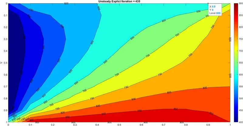
RESULTS & DISCUSSIONS:
- In steady state methods, there is no time loop and the results converge within a few iterations.We include time loop for implicit methods and it runs for a large number of iterat ions.
- Transient solvers take a lot of time for computation as it is a funct ion of both time and position, when comparing to steady state solver which is only a funct ion of position .
- The SOR provides us the answer with less number of iterations and takes less computation time.
CONCLUSION:
The 2D heat conduction equation was solved making use of iterative techniques.