OBJECTIVE:

Derive the following 4th order approximations of the second-order derivative.

1. Central difference

2. Skewed right-sided difference

3. Skewed left-sided difference

4. Prove that skewed schemes are fourth-order accurate i.e the thumb rule.

5. Write a program in Matlab to evaluate the second-order derivative of the analytical function exp(x)*cos(x) and compare it with the 3 numerical approximations that have been derived.

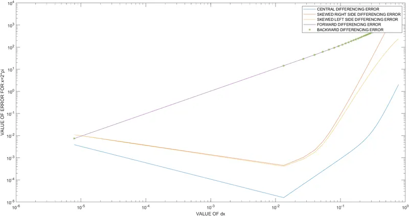
6. Provide a plot that compares the absolute error between the above-mentioned schemes.

7. Describe why a skewed scheme is useful? What can a skewed scheme do that a CD(Central difference) scheme cannot?

PROBLEM FORMULATION & METHODOLOGY:

CENTRAL DIFFERENCE:

NUMBER OF NODES

The number of nodes(N) = P+Q-1 , for central difference scheme.

In the above Eqn, we have N=The number of nodes;P=The order of derivative=2; Q=order of approximation=4

N=2+4-1=5,Hence N=5

DERIVATION:

To derive fourth order approximation for the second order derivative, we start with the following approximation.

`(dx^2)(∂^2 f)/(∂x^2 )≅af(i-2)+b(i-1)+c(i)+d(i+1)+e(i+2)` .....................(1a)

Hence, we have

`(∂^2 f)/(∂x^2 )≅({af(i-2)+b(i-1)+c(i)+d(i+1)+e(i+2)})/((dx^2))` ....................(2a)

Hence, we can expand all the terms in Eqn(1a) from the following table (TAYLOR's TABLE)

TERMS IN THE Eqn (A)	f(i)	`∆xf^1 (x)`	`∆x^2 f^2 (x)`	`∆x^3 f^3 (x)`	`∆x^4 f^4 (x)`	`∆x^5 f^5 (x)`
af(i-2)	a	-2a	`(4a)/2`	`(-8a)/6`	`(16a)/24`	`(-32a)/120`
bf(i-1)	b	-b	`b/2`	`-b/6`	`b/24`	`-b/120`
cf(i)	c	0	0	0	0	0
df(i+1)	d	d	`d/2`	`d/6`	`d/24`	`d/120`
ef(i+2)	e	2e	`(4e)/2`	`(8e)/6`	`(16e)/24`	`(-32a)/120`
`∑A`= af(i-2)+ bf(i-1)+cf(i)+df(i+1)+ef(i+2)	0	0	1	0	0	`Κ`

Where `Κ` is some constant

Now, from the above TAYLOR's TABLE, we get the following Eqns.

a+b+c+d+e=0 ................(1)

-2a-b+0+d+2e=0 ....................(2)

`(4a)/2`+ `b/2`+0+`d/2`+`(4e)/2`=1 ................(3)

`(-8a)/6`+`-b/6`+0+`d/6`+`(8e)/6`=0 ................(4)

`(16a)/24`+`b/24`+0+`d/24`+`(16e)/24`=0 ...........(5)

We will convert the following above Eqn (1),(2),(3),(4),(5) in the matrix form i.e. A*X=B .

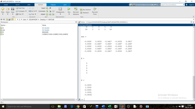
Where A=`[[1,1,1,1,1],[-2,-1,0,1,2],[4,1,0,1,4],[-8,-1,0,1,8],[16,1,0,1,16]]`, X=`[[a] ,[b],[c],[d],[e]]`, B=`[[0],[0],[2],[0],[0]]`

Hence, we have X=inv(A)*B, Hence X=`[[-0.0833 ] , [1.3333] , [-2.5000] , [1.3333] , [-0.0833]]`

From the above matrix it is a=e & b=d. Hence, substituting the Eqn in Eqn (2a) we get: `(∂^2 f)/(∂x^2 )≅({-0.0833f(i-2)+1.3333(i-1)-2.5000(i)+1.3333(i+1)-0.0833(i+2)})/((dx^2))`

MATLAB WORKSPACE & COMMAND WINDOW:

PROOF OF FOURTH ORDER ERROR:

We shall expand the TAYLOR'S TABLE terms[we shall include the heigher order terms]

`(dx^2)(∂^2 f)/(∂x^2 )`=`{4a+b+0+d+4e}f^2 (x)(dx^2)/(2!)`+`{-32a-b+0+d+4e}f^5 (x)(dx^5)/(5!)`+`{64a+b+0+d+64e}f^6 (x)(dx^6)/(6!)`+ ..........

We know that the coefficient of `f^2(x)` is 1, again since a=e & b=d the fifth term will be O. Hence, we get

`(dx^2)(∂^2 f)/(∂x^2 )`=`{4a+b+0+d+4e}f^2 (x)(dx^2)/(2!)` + O +`{64a+b+0+d+64e}f^6 (x)(dx^6)/(6!)`+......

Now, we substitue the value of `(dx^2)(∂^2 f)/(∂x^2 )` we get from Eqn(1a)

`({af(i-2)+b(i-1)+c(i)+d(i+1)+e(i+2)})` =`{4a+b+0+d+4e}f^2 (x)(dx^2)/(2!)` + O +`{64a+b+0+d+64e}f^6 (x)(dx^6)/(6!)`+....

Now, we devide the above Eqn by `(dx^2)` we get:

`({af(i-2)+b(i-1)+c(i)+d(i+1)+e(i+2)})/((dx^2))`=`{4a+b+0+d+4e}f^2 (x)/(2!)` + O +`{64a+b+0+d+64e}f^6 (x)(dx^4)/(6!)`+....

Hence, in RHS we have the term `{64a+b+0+d+64e}f^6 (x)(dx^4)/(6!)`=O`(dx^4)`

Hence, we have the Required Eqn as:

`({af(i-2)+b(i-1)+c(i)+d(i+1)+e(i+2)})/((dx^2))`= `{4a+b+0+d+4e}f^2 (x)/(2!)`+ O`(dx^4)`

Hence, this is prooved that the CENTRAL DIFFERENCE SCHEME is of fourth-order accurate.

SKEWED RIGHT-SIDE DIFFERENCE:

NUMBER OF NODES

The number of nodes(N) = P+Q , for Skewed right-sided difference.

In the above Eqn, we have N=The number of nodes;P=The order of derivative=2; Q=order of approximation=4

N=2+4=6,Hence N=6

DERIVATION:

To derive fourth order approximation for the second order derivative, we start with the following approximation.

`(dx^2)(∂^2 f)/(∂x^2 )≅af(i)+bf(i+1)+cf(i+2)+df(i+3)+ef(i+4)+hf(i+5)` .....................(1a)

Hence, we have

`(∂^2 f)/(∂x^2 )≅({af(i)+bf(i+1)+cf(i+2)+df(i+3)+ef(i+4)+hf(i+5)})/((dx^2))` ....................(2a)

Hence, we can expand all the terms in Eqn(1a) from the following table (TAYLOR's TABLE)

TERMS IN THE Eqn (A)	f(i)	`∆xf^1 (x)`	`∆x^2 f^2 (x)`	`∆x^3 f^3 (x)`	`∆x^4 f^4 (x)`	`∆x^5 f^5 (x)`	`∆x^6 f^6(x)`
af(i)	a	0	0	0	0	0	0
bf(i+1)	b	b	b	b	b	b	b
cf(i+2)	c	2c	4c	8c	16c	32c	64c
df(i+3)	d	3d	9d	27d	81d	243d	729d
ef(i+4)	e	4e	16e	64e	256e	1024e	4096e
hf(i+5)	h	5h	25h	125h	625h	3125h	15625h
`∑A`=af(i)+bf(i+1)+cf(i+2)+df(i+3)+ef(i+4)+hf(i+5)	0	0	1	0	0	0	`Κ`

Where `Κ` is some constant

Now, from the above TAYLOR's TABLE, we get the following Eqns.

a+b+c+d+e+h=0 ................(1)

0+b+2c+3d+4e+5h=0 ....................(2)

(0+b+4c+9d+16e+25h)/2=1 ....................(3)

0+b+8c+27d+64e+125h=0 ................(4)

0+b+16c+81d+256e+625h=0 ....................(5)

0+b+32c+243d+1024e+3125h=0 ...........(6)

We will convert the following above Eqn (1),(2),(3),(4),(5),(6) in the matrix form i.e. A*X=B .

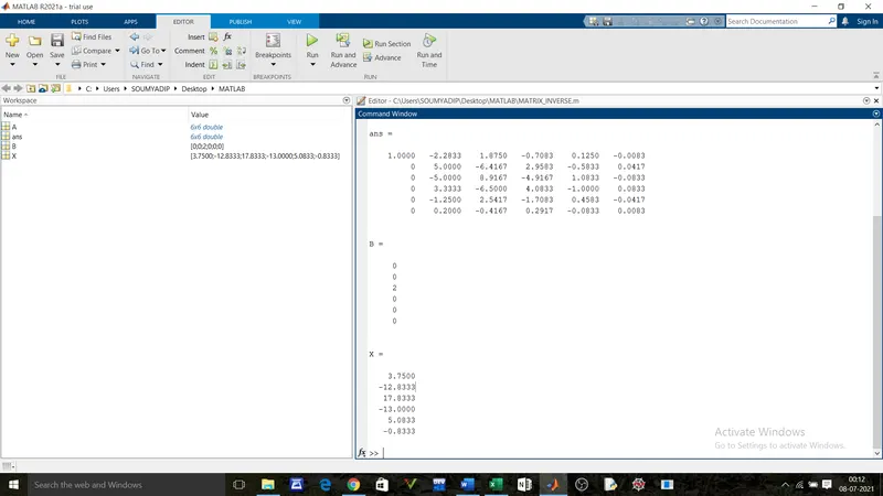
Where A=`[[1,1,1,1,1,1],[0,1,2,3,4,5],[0,1,4,9,16,25],[0,1,8,27,64,125],[0,1,16,81,256,625],[0,1,32,243,1024,3125]]`; X=`[[a] ,[b],[c],[d],[e],[h]]`; B=`[[0],[0],[2],[0],[0],[0]]`

Hence, we have X=inv(A)*B, Hence X=`[[ 3.7500],[-12.8333],[17.8333],[-13.0000],[5.0833],[-0.8333]]`

Hence, substituting the Eqn in Eqn (2a) we get: `(∂^2 f)/(∂x^2 )≅({3.7500f(i)-12.8333(i+1)+17.8333(i+2)-13.0000(i+3)+5.0833(i+4)-0.8333f(i+5)})/((dx^2))`

MATLAB WORKSPACE & COMMAND WINDOW:

PROOF OF FOURTH ORDER ERROR FOR SKEWED RIGHT-SIDE DIFFERENCE:

We shall expand the TAYLOR'S TABLE terms[we shall include the heigher order terms]

`(dx^2)(∂^2 f)/(∂x^2 )`=`{(0+b+4c+9d+16e+25h)}f^2 (x)(dx^2)/(2!)`+`{0+b+32c+243d+1024e+3125h}f^5 (x)(dx^5)/(5!)`+`{0+b+64c+729d+4096e+15625h}f^6 (x)(dx^6)/(6!)`+ ..........

The fifth term will be O. Hence, we get

`(dx^2)(∂^2 f)/(∂x^2 )`=`{0+b+4c+9d+16e+25h}f^2 (x)(dx^2)/(2!)` + O +`{0+b+64c+729d+4096e+15625h}f^6 (x)(dx^6)/(6!)`+......

Now, we substitue the value of `(dx^2)(∂^2 f)/(∂x^2 )` we get from Eqn(1a)

`({af(i)+bf(i+1)+cf(i+2)+df(i+3)+ef(i+4)+hf(i+5)})` =`{0+b+4c+9d+16e+25h}f^2 (x)(dx^2)/(2!)` + O +`{0+b+64c+729d+4096e+15625h}f^6 (x)(dx^6)/(6!)`+....

Now, we devide the above Eqn by `(dx^2)` we get:

`({af(i)+bf(i+1)+cf(i+2)+df(i+3)+ef(i+4)+hf(i+5)})/((dx^2))`=`{0+b+4c+9d+16e+25h}f^2 (x)/(2!)` + O +`{0+b+64c+729d+4096e+15625h}f^6 (x)(dx^4)/(6!)`+....

Hence, in RHS we have the term `{0+b+64c+729d+4096e+15625h}f^6 (x)(dx^4)/(6!)`=O`(dx^4)`

Hence, we have the Required Eqn as:

`({af(i)+bf(i+1)+cf(i+2)+df(i+3)+ef(i+4)+hf(i+5)})/((dx^2))`= `{0+b+4c+9d+16e+25h}f^2 (x)/(2!)`+ O`(dx^4)`

Hence, this is prooved that the SKEWED RIGHT-SIDE DIFFERENCE is of fourth-order accurate.

SKEWED LEFT-SIDE DIFFERENCE:

NUMBER OF NODES

The number of nodes(N) = P+Q , for Skewed right-sided difference.

In the above Eqn, we have N=The number of nodes;P=The order of derivative=2; Q=order of approximation=4

N=2+4=6,Hence N=6

DERIVATION:

To derive fourth order approximation for the second order derivative, we start with the following approximation.

`(dx^2)(∂^2 f)/(∂x^2 )≅af(i-5)+bf(i-4)+cf(i-3)+df(i-2)+ef(i-1)+hf(i)` .....................(1a)

Hence, we have

`(∂^2 f)/(∂x^2 )≅({af(i-5)+bf(i-4)+cf(i-3)+df(i-2)+ef(i-1)+hf(i)})/((dx^2))` ....................(2a)

Hence, we can expand all the terms in Eqn(1a) from the following table (TAYLOR's TABLE)

TERMS IN THE Eqn (A)	f(i)	`∆xf^1 (x)`	`∆x^2 f^2 (x)`	`∆x^3 f^3 (x)`	`∆x^4 f^4 (x)`	`∆x^5 f^5 (x)`	`∆x^6 f^6(x)`
af(i-5)	a	-5a	25a	-125a	625a	-3125a	15625a
bf(i-4)	b	-4b	16b	-64b	256b	-1024b	4096b
cf(i-3)	c	-3c	9c	-27c	81c	-243c	729c
df(i-2)	d	-2d	4d	-8d	16d	-32d	64d
ef(i-1)	e	-e	e	-e	e	-e	e
hf(i)	h	0	0	0	0	0	0
`∑A`=af(i-5)+bf(i-4)+cf(i-3)+df(i-2)+ef(i-1)+hf(i)	0	0	1	0	0	0	`Κ`

Where `Κ` is some constant

Now, from the above TAYLOR's TABLE, we get the following Eqns.

a+b+c+d+e+h=0 ................(1)

-5a-4b-3c-2d-e+0=0 ....................(2)

(25a+16b+9c+4d+e+0)/2=1 ....................(3)

-125a-64b-27c-8d-e+0=0 ................(4)

625a+256b+81c+16d+e+0=0 ....................(5)

-3125a-1024b-243c-32d-e+0=0 ...........(6)

We will convert the following above Eqn (1),(2),(3),(4),(5),(6) in the matrix form i.e. A*X=B .

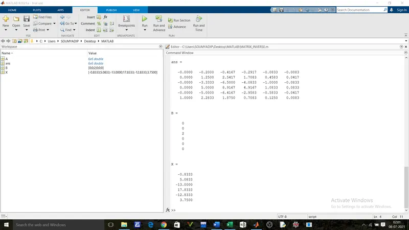
Where A=`[[1,1,1,1,1,1],[-5,-4,-3,-2,-1,0],[25,16,9,4,1,0],[-125,-64,-27,-8,-1,0],[625,256,81,16,1,0],[-3125,-1024,-243,-32,-1,0]]`; X=`[[a] ,[b],[c],[d],[e],[h]]`; B=`[[0],[0],[2],[0],[0],[0]]`

Hence, we have X=inv(A)*B, Hence X=`[[ -0.8333],[5.0833],[-13.0000],[17.8333],[-12.8333],[3.7500]]`

Hence, substituting the Eqn in Eqn (2a) we get: `(∂^2 f)/(∂x^2 )≅({-0.8333f(i)+5.0833(i+1)-13.0000(i+2)+17.8333(i+3)-12.8333(i+4)+3.7500f(i+5)})/((dx^2))`

MATLAB WORKSPACE & COMMAND WINDOW:

PROOF OF FOURTH ORDER ERROR FOR SKEWED LEFT-SIDE DIFFERENCE:

We shall expand the TAYLOR'S TABLE terms[we shall include the heigher order terms]

`(dx^2)(∂^2 f)/(∂x^2 )`=`{(25a+16b+9c+4d+e+0)}f^2 (x)(dx^2)/(2!)`+`{-3125a-1024b-243c-32d-e+0}f^5 (x)(dx^5)/(5!)`+`{15625a+4096b+729c+64d+e+0}f^6 (x)(dx^6)/(6!)`+ ..........

The fifth term will be O. Hence, we get

`(dx^2)(∂^2 f)/(∂x^2 )`=`{25a+16b+9c+4d+e+0}f^2 (x)(dx^2)/(2!)` + O +`{15625a+4096b+729c+64d+e+0}f^6 (x)(dx^6)/(6!)`+......

Now, we substitue the value of `(dx^2)(∂^2 f)/(∂x^2 )` we get from Eqn(1a)

`({af(i-5)+bf(i-4)+cf(i-3)+df(i-2)+ef(i-1)+hf(i)})` =`{25a+16b+9c+4d+e+0}f^2 (x)(dx^2)/(2!)` + O +`{15625a+4096b+729c+64d+e+0}f^6 (x)(dx^6)/(6!)`+....

Now, we devide the above Eqn by `(dx^2)` we get:

`({af(i-5)+bf(i-4)+cf(i-3)+df(i-2)+ef(i-1)+hf(i)})/((dx^2))`=`{25a+16b+9c+4d+e+0}f^2 (x)/(2!)` + O +`{15625a+4096b+729c+64d+e+0}f^6 (x)(dx^4)/(6!)`+....

Hence, in RHS we have the term `{15625a+4096b+729c+64d+e+0}f^6 (x)(dx^4)/(6!)`=O`(dx^4)`

Hence, we have the Required Eqn as:

`({af(i-5)+bf(i-4)+cf(i-3)+df(i-2)+ef(i-1)+hf(i)})/((dx^2))`= `{25a+16b+9c+4d+e+0}f^2 (x)/(2!)`+ O`(dx^4)`

Hence, this is prooved that the SKEWED LEFT-SIDE DIFFERENCE is of fourth-order accurate.

MATLAB CODE TO EVALUTE THE SECOND ORDER DERIVATIVE OF THE ANALYTICAL FUNCTION exp(x)*cos(x) & COMPARE IT WITH THE PREVIOUS 3 NUMERICAL APPROXIMATION:

% Computation of heigher order approximations using symmetric & skewed 
% Stencils for the function, f(x)=exp(x)*cos(x)
% We assume the suitable variables x & dx
x=2*pi;
dx=linspace(pi/4,pi/400000,60);
% Declaration of the size of the variavles
cd_error=zeros(1,length(dx));
srd_error=zeros(1,length(dx));
sld_error=zeros(1,length(dx));
fwd_error=zeros(1,length(dx));
bwd_error=zeros(1,length(dx));
% Getting the analytical solution for the function f''(x)=-2*exp(x)*sin(x)
act_solution=-2*exp(x)*sin(x);
% Loop to compute various numerical solution for each dx
for i=1:length(dx)
    f=exp(x)*cos(x);                           %f(x)
    f1=exp(x+dx(i))*cos(x+dx(i));              %f(x+1)
    f2=exp(x+2*dx(i))*cos(x+2*dx(i));          %f(x+2)
    f3=exp(x+3*dx(i))*cos(x+3*dx(i));          %f(x+3)
    f4=exp(x+4*dx(i))*cos(x+4*dx(i));          %f(x+4)
    f5=exp(x+5*dx(i))*cos(x+5*dx(i));          %f(x+5)
    f1m=exp(x-dx(i))*cos(x-dx(i));             %f(x-1)
    f2m=exp(x-2*dx(i))*cos(x-2*dx(i));         %f(x-2)
    f3m=exp(x-3*dx(i))*cos(x-3*dx(i));         %f(x-3)
    f4m=exp(x-4*dx(i))*cos(x-4*dx(i));         %f(x-4)
    f5m=exp(x-5*dx(i))*cos(x-5*dx(i));         %f(x-5)
    % Computing solutions of f(x) using various differencing schemes
    % Calling the representative functions
    cd_solution=central_difference(f2m,f1m,f,f1,f2,dx(i));
    srd_solution=skewed_right_difference(f,f1,f2,f3,f4,f5,dx(i));
    sld_solution=skewed_left_difference(f5m,f4m,f3m,f2m,f1m,f,dx(i));
    fwd_solution=forward_difference(f,f1,f2,dx(i));
    bwd_solution=backward_difference(f2,f1,f,dx(i));
    % Calculation of absolute error of each of the differencing scheme 
    cd_error(i)=abs(act_solution-cd_solution);
    srd_error(i)=abs(act_solution-srd_solution);
    sld_error(i)=abs(act_solution-sld_solution);
    fwd_error(i)=abs(act_solution-fwd_solution);
    bwd_error(i)=abs(act_solution-bwd_solution);
end
% Graph plotting between dx and various differencing schemes
figure(1)
loglog(dx,cd_error,dx,srd_error,dx,sld_error,dx,fwd_error,dx,bwd_error,'*');
xlabel('VALUE OF dx');
ylabel('VALUE OF ERROR FOR x=2*pi');
legend('CENTRAL DIFFERENCING ERROR','SKEWED RIGHT SIDE DIFFERENCING ERROR','SKEWED LEFT SIDE DIFFERENCING ERROR','FORWARD DIFFERENCING ERROR','BACKWARD DIFFERENCING ERROR') 
% Function defination for CENTRAL DIFFERENCE APPROXIMATION:
function cd_solution=central_difference(f2m,f1m,f,f1,f2,dx)
%VALUES DERIVED FROM TAYLOR'S TABLE
a=-0.0833;
b=1.3333;
c=-2.5000;
d=1.3333;
e=-0.0833;
% Central difference scheme for the 4th order solution to 2nd order derivative:
cd_solution=(a*f2m+b*f1m+c*f+d*f1+e*f2)/dx^2;
end
% Function defination for SKEWED  RIGTH SIDE DIFFERENCE APPROXIMATION:
function srd_solution=skewed_right_difference(f,f1,f2,f3,f4,f5,dx)
%VALUES DERIVED FROM TAYLOR'S TABLE
a=3.75000;
b=-12.83333;
c=17.83333;
d=-13.00000;
e=5.08333;
h=-0.83333;
% Skewed right side scheme for the 4th order solution to 2nd order derivative:
srd_solution=(a*f+b*f1+c*f2+d*f3+e*f4+h*f5)/dx^2;
end
% Function defination for SKEWED  LEFH SIDE DIFFERENCE APPROXIMATION:
function sld_solution=skewed_left_difference(f5m,f4m,f3m,f2m,f1m,f,dx)
%VALUES DERIVED FROM TAYLOR'S TABLE
a=-0.83333;
b=5.08333;
c=-13.00000;
d=17.83333;
e=-12.83333;
h=3.75000;
% Skewed right side scheme for the 4th order solution to 2nd order derivative:
sld_solution=(a*f5m+b*f4m+c*f3m+d*f2m+e*f1m+h*f)/dx^2;
end
% Function defination for FORWARD DIFFERENCE APPROXIMATION:
function fwd_solution=forward_difference(f,f1,f2,dx)
%VALUES DERIVED FROM TAYLOR'S TABLE
%a=
%b=
%c=
% Skewed right side scheme for the 4th order solution to 2nd order derivative:
fwd_solution=(f-2*f1+f2)/dx^2;
end
% Function defination for BACKWARD DIFFERENCE APPROXIMATION:
function bwd_solution=backward_difference(f2,f1,f,dx)
%VALUES DERIVED FROM TAYLOR'S TABLE
%a=
%b=
%c=
% Skewed right side scheme for the 4th order solution to 2nd order derivative:
bwd_solution=(f2-2*f1+f)/dx^2;
end

   
 

OUTPUT FIGURE(PLOT):

WORKSPACE:

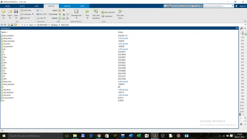
Inference:

From the above comparison of different schemes for fourth order approximation of a second-order derivative, we can reassure that the central difference approx imation yields more accurate solutions than the right-skewed and left-skewed differencingschemes.Since forward and backward approximations are of second-order error, they give out larger errors than the other fourth-order schemes.

It may also be noted that if we consider a wider range of dx, at some values of dx, the error produced by higher order schemes is bigger than that of the lower order schemes.This is due to higher roundoff errors at those points. It is important to understand that the value of error at any point is the net sum of numerical error and roundoff error and the round off error increases with increase in the order of error.Therefore, a higher-order scheme may not be always desirable.

Significance of a skewed scheme:

A function is always characterized by a domain.A domain is a space or area beyond which a function ceases to exist. Therefore a domain has boundaries and the function exists on only one side of the boundary. Now, if we want to compute a numericalapprox imation for the funct ion at the boundary,we cannot use a centraldifference scheme as it requires data from both sides of the boundary.That is where a skewed difference scheme plays a vitalrole since data from any side can be used to perform numerical approximation at a point.