Week 5.1 - Mid term project - Solving the steady and unsteady 2D heat conduction problem
The 2D Diffusion equation obtained from General Scalar Transport equation, with no source terms,
`(delT)/(delt)=alpha((del^2T)/(delx^2)+(del^2T)/(dely^2))` - Transient heat conduction.
As `t->oo`, `(del^2T)/(delx^2)+(del^2T)/(dely^2)=0` - Steady state heat conduction
The 2D Diffusion equation is solved on a square plate of unit dimensions and the heat equation is discretized using second order central difference scheme for spatial derivatives and first order forward difference scheme for temporal derivative.
`(delT)/(delt)=(T^((n+1))-T^((n)))/(Deltat)`, here `T^((n+1))` denotes value of temperature at the next time step, while `T^((n))` denotes the value at current time step.
`(del^2T)/(delx^2)= (T(i+1,j)-2T(i,j)+T(i-1,j))/(Deltax^2)`
`(del^2T)/(dely^2)= (T(i,j+1)-2T(i,j)+T(i,j-1))/(Deltay^2)`
Therefore, `(del^2T)/(delx^2)+(del^2T)/(dely^2)= (T(i+1,j)-2T(i,j)+T(i-1,j))/(Deltax^2)+(T(i,j+1)-2T(i,j)+T(i,j-1))/(Deltay^2)`.
`(delT)/(delt)=alpha((del^2T)/(delx^2)+(del^2T)/(dely^2))`.
`->(T^((n+1))-T^((n)))/(Deltat)=alpha( (T(i+1,j)-2T(i,j)+T(i-1,j))/(Deltax^2)+(T(i,j+1)-2T(i,j)+T(i,j-1))/(Deltay^2))`.
The transient state heat conduction equation can be evaluated at two different time steps.
The heat equation evaluated at `n`th time step is called explicit scheme because the Temperature value at the next time step can be explicitly expressed as the values of temperatures of neighbouring nodes at the previous time step.
`T^((n+1))=(Deltat)alpha( (T^(n)(i+1,j)-2T^(n)(i,j)+T^(n)(i-1,j))/(Deltax^2)+(T^(n)(i,j+1)-2T^(n)(i,j)+T^(n)(i,j-1))/(Deltay^2))+T^((n))`.
while the same equation evaluated at `(n+1)`th time step is called implicit scheme.
`T^((n+1))=(Deltat)alpha( (T^(n+1)(i+1,j)-2T^(n+1)(i,j)+T^(n+1)(i-1,j))/(Deltax^2)+(T^(n+1)(i,j+1)-2T^(n+1)(i,j)+T^(n+1)(i,j-1))/(Deltay^2))+T^((n))`.
The steady state heat conduction equation and transient implicit scheme requires linear solvers to obtain the Temperature profile.
- Jacobi iterative method.
- Gauss-seidel method.
- Successive Over Relaxation(SOR) method.
Jacobi Algorithm:
`x_i^((k+1))=1/a_(ii)(b_i-sum_(jnei)^n a_(ij) *x_j^((k))) , i=1,2,3,..n`
Gauss-Seidel Algorithm:
`x_i^((k+1))=1/a_(ii)(b_i-sum_(j=1)^(i-1) a_(i) *x_j^((k))-sum_(i=i+1)^n a_(ij) *x_j^((k))) , i=1,2,3,..n`
Successive Over Relaxation:
`T_i^((k+1))= (1-w)T_i^((k))+w(x_(jacobi)^(k+1) or x_(gauss-seidelel))^(k+1)`
Code:
Steady state heat conduction:
close all
clc
method=(input('Enter choice of linear solver: 1->Jacobi,2->Gauss-siedel,3->Successive Over Relaxation\n'));
L=1;                                      % Length and breadth of the domain
px=linspace(0,1,100);                     % Mesh generation along x
py=px;                                    % Mesh generation along y
nx=length(px);                            % Number of grid points along x
ny=nx;                                    % Number of grid points along y
dx=px(2)-px(1);                           % grid spacing along x-> dx
dy=dx;                                    % grid spacing along y-> dy
Tmat=ones(length(px),length(py))*((400+800+600+900)/4); % Initializing all the elements of temperature matrix
Tmat(:,1)=400;                            % Boundary condition left end of the plate
Tmat(:,end)=800;                          % Boundary condition right end of the plate
Tmat(1,:)=600;                            % Boundary condition top end of the plate
Tmat(end,:)=900;                          % Boundary condition bottom end of the plate
Tmat(1,1)=(400+600)/2;                    % Averaging the conditions at top left corner
Tmat(end,1)=(400+900)/2;                  % Averaging the conditions at bottom left corner
Tmat(1,end)=(600+800)/2;                  % Averaging the conditions at top right edge corner
Tmat(end,end)=(900+800)/2;                % Averaging the conditions at bottom right corner
error=1e4;                                % Error tolerance
count=0;                                  % Initial count
Tmat_n=Tmat;                              % Copying initial Temperature matrix
w=1.9;                                    % Defining weights for SOR-Successive over relaxation method

if method==1                              % if method==1 then Jacobi is implemented
while error>1e-4                          % Keep iterating the below procedure till error drops below 10^-4
 for i=2:nx-1                             % Travelling along the 'x' direction of the domain
    for j=2:ny-1                          % Travelling along the 'y' direction of the domain
        Tmat_n(i,j)=((dy)^2*(Tmat(i+1,j)+Tmat(i-1,j))+(dx)^2*(Tmat(i,j+1)+Tmat(i,j-1)))/(2*((dx)^2+(dy)^2)); % Discretized Laplacian of Temperature
    end
 end
 error=max(max(abs(Tmat_n-Tmat)));        % Defining error as maximum of absolute difference between present matrix and previously iterated matrix
 Tmat=Tmat_n;                             % Updating the matrix to serve current iterated matrix as new guess matrix
 count=count+1;                           % Updating the count value
end
   imagesc(Tmat)                          % Heatmap of Temperature profile of domain
   colormap(jet);                         % choosing color for heatmap
   colorbar;                              % Colorbar to display color to number relationship
   xlabel('Grid points along x')          % Labelling x axis
   ylabel('Grid points along y')          % Labelling y axis
   title({'Steady state heat conduction'},{sprintf('Jacobi iteration count = %d',count)}) % Title for the graph
   fprintf('Number of iterations to reach below tolerance=%d\n',count)% Printing count
end

if method==2                              % if method==1 then Jacobi is implemented
    while error>1e-4                      % Keep iterating the below procedure till error drops below 10^-4
        for i=2:nx-1                      % Travelling along the 'x' direction of the domain
            for j=2:ny-1                  % Travelling along the 'y' direction of the domain
                Tmat_n(i,j)=((dy)^2*(Tmat(i+1,j)+Tmat_n(i-1,j))+(dx)^2*(Tmat(i,j+1)+Tmat_n(i,j-1)))/(2*((dx)^2+(dy)^2)); % Discretized Laplacian of Temperature
            end
        end
      error=max(max(abs(Tmat_n-Tmat)));   % Defining error as maximum of absolute difference between present matrix and previously iterated matrix
      Tmat=Tmat_n;                        % Updating the matrix to serve current iterated matrix as new guess matrix
      count=count+1;                      % Updating the count value
    end
   imagesc(Tmat)                          % Heatmap of Temperature profile of domain
   colormap(jet);                         % choosing color for heatmap
   colorbar;                              % Colorbar to display color to number relationship
   xlabel('Grid points along x')          % Labelling x axis
   ylabel('Grid points along y')          % Labelling y axis
   title({'Steady state heat conduction'},{sprintf('Gauss-Seidel iteration count = %d',count)}) % Title for the graph
   fprintf('Number of iterations to reach below tolerance=%d\n',count) % Printing count
end

if method==3                              % if method==3 then SOR(successive over relaxation) is implemented
    while error>1e-4                      % Keep iterating the below procedure till error drops below 10^-4
        for i=2:nx-1                      % Travelling along the 'x' direction of the domain
            for j=2:ny-1                  % Travelling along the 'y' direction of the domain
                Tmat_n(i,j)=Tmat(i,j)*(1-w)+w*(((dy)^2*(Tmat(i+1,j)+Tmat_n(i-1,j))+(dx)^2*(Tmat(i,j+1)+Tmat_n(i,j-1)))/(2*((dx)^2+(dy)^2))); % Discretized Laplacian of Temperature
            end
        end
        error=max(max(abs(Tmat_n-Tmat))); % Defining error as maximum of absolute difference between present matrix and previously iterated matrix
      Tmat=Tmat_n;                        % Updating the matrix to serve current iterated matrix as new guess matrix
      count=count+1;
    end
   imagesc(Tmat);                         % Heatmap of Temperature profile of domain
   colormap(jet);                         % choosing color for heatmap
   colorbar;                              % Colorbar to display color to number relationship
   xlabel('Grid points along x')          % Labelling x axis
   ylabel('Grid points along y')          % Labelling y axis
   title({'Steady state heat conduction'},{[sprintf('SOR iteration count = %d',count)],[' Relaxation factor w=' num2str(w)]}) % Title for the graph
   fprintf('Number of iterations to reach below tolerance=%d\n',count) % Printing count
end
The code is self-explanatory, the comments describes the function of each line of code.
Outputs:
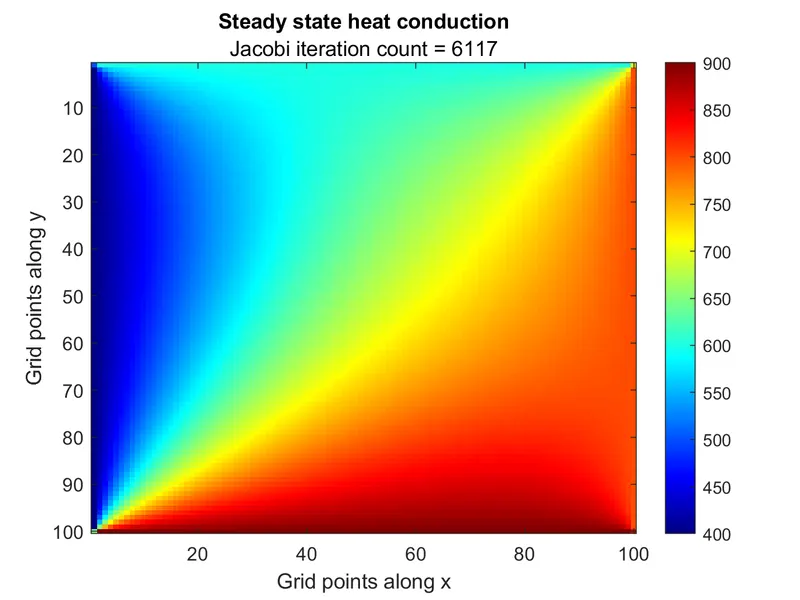
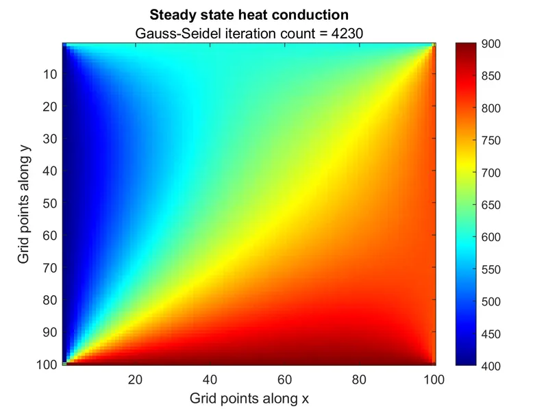
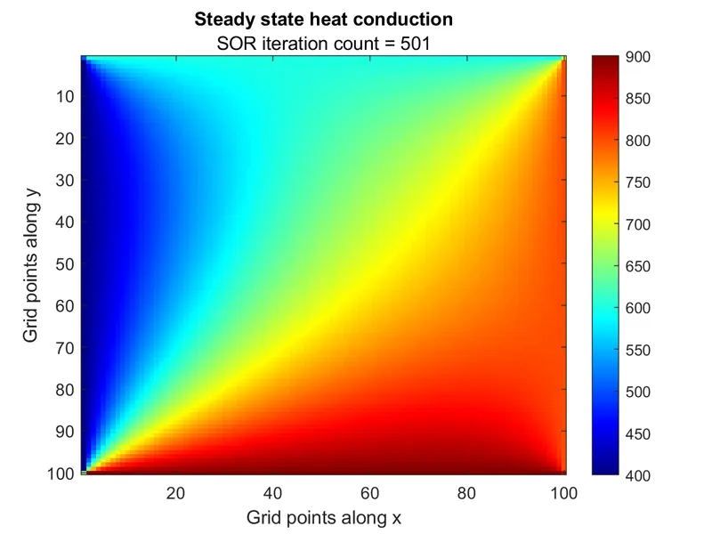
SOR with weighting factor,w=1.9;
Code:
The transient state explicit solution:
close all
clc
tic
L=1;                                % Length and breadth of the domain
px=linspace(0,1,70);                % Grid generation along x
py=px;                              % Grid generation along y
nx=length(px);                      % Number of grid points along x
ny=nx;                              % Number of grid points along y
dx=px(2)-px(1);                     % grid spacing along x-> dx
dy=dx;                              % grid spacing along y-> dy
Tmat=ones(length(px),length(py));   % Initializing all the elements of temperature matrix
Tmat(:,1)=400;                      % Boundary condition left end of the plate
Tmat(:,end)=800;                    % Boundary condition right end of the plate
Tmat(1,:)=600;                      % Boundary condition top end of the plate
Tmat(end,:)=900;                    % Boundary condition bottom end of the plate
Tmat(1,1)=(400+600)/2;              % Averaging the conditions at top left corner
Tmat(end,1)=(400+900)/2;            % Averaging the conditions at bottom left corner
Tmat(1,end)=(600+800)/2;            % Averaging the conditions at top right edge corner
Tmat(end,end)=(900+800)/2;          % Averaging the conditions at bottom right corner
Tmat_n=Tmat;                        % Copying initial Temperature matrix
alpha=3.05;                         % Defining thermal diffusivity of the material
dt=1.7e-5;                          % Defining time step
k1=(alpha*dt/(dx^2));               % CFL1
k2=(alpha*dt/(dy^2));               % CFL2
t=0;
%%%% Explicit method %%%%%

for nt=1:1e5                        % Time loop
        for i=2:nx-1                % Travelling along 'x' direction of the domain
            for j=2:ny-1            % Travelling along 'y' direction of the domain
                Tmat(i,j)=Tmat(i,j)+k1*(Tmat(i-1,j)-2*Tmat(i,j)+Tmat(i+1,j))+k2*(Tmat(i,j+1)-2*Tmat(i,j)+Tmat(i,j-1)); % Explicit form of the heat equation
            end
        end
        t=t+dt;
end
imagesc(Tmat);                      % To plot temperature profile
colormap(jet);                      % choosing color for heatmap
ylabel('Grid points along y');      % Label y axis
xlabel('Grid points along x');      % Label x axis
title({'Unsteady diffusion-Explicit scheme'},{['CFL1=CFL2=(\alpha\Delta t/\Delta x^2) = ' num2str(k1)],[' time= ' num2str(t)]}); % Title of the plot
colorbar                            % To display colorbar
toc
Here,
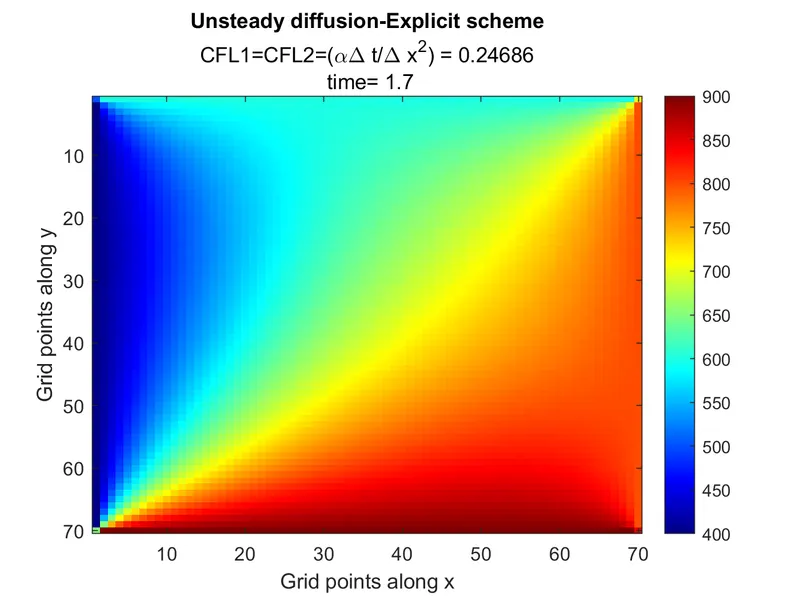
`CFL1=CFL2=alpha(Deltat)/(Deltax)^2=alpha(Deltat)/(Deltay)^2`.
`CFL1+CFL2<=0.5` is satisfied so a stable solution is obtained. Also CFL1=CFL2 because `Delta x=Deltay`.
Outputs:
Code:
Transient implicit solution:
clear all
close all
clc
method=(input('Enter choice of linear solver: 1->Jacobi,2->Gauss-siedel,3->Successive Over Relaxation\n'));
L=1;                                      % Length and breadth of the domain
px=linspace(0,1,100);                     % Grid generation along x
py=px;                                    % Grid generation along y
nx=length(px);                            % Number of grid points along x
ny=nx;                                    % Number of grid points along y
dx=px(2)-px(1);                           % Grid spacing along x-> dx
dy=dx;                                    % Grid spacing along y-> dy
Tmat=ones(length(px),length(py))*((400+800+600+900)/4); % Initializing all the elements of temperature matrix
Tmat(:,1)=400;                            % Boundary condition left end of the plate
Tmat(:,end)=800;                          % Boundary condition right end of the plate
Tmat(1,:)=600;                            % Boundary condition top end of the plate
Tmat(end,:)=900;                          % Boundary condition bottom end of the plate
Tmat(1,1)=(400+600)/2;                    % Averaging the conditions at top left corner
Tmat(end,1)=(400+900)/2;                  % Averaging the conditions at bottom left corner
Tmat(1,end)=(600+800)/2;                  % Averaging the conditions at top right edge corner
Tmat(end,end)=(900+800)/2;                % Averaging the conditions at bottom right corner
error=1e4;                                % Error tolerance
count=0;                                  % Initial count
Tmat_n=Tmat;                              % Copying initial Temperature matrix
alpha=3;                                  % Defining thermal diffusivity of the material
dt=1.7e-2;                                % Defining time step
k1=(alpha*dt/(dx^2));                     % CFL 1
k2=(alpha*dt/(dy^2));                     % CFL 2
k=(1+2*k1+2*k2);
T_pres=Tmat;
TGS=Tmat;
t=0;                                      % initializing time
w=1.9;                                    % weighting factor for SOR


%%%%% Implicit method %%%%%

if method==1                              % Jacobi
 for nt=1:1e2                             % Time loop
    while error>1e-4                      % Keep iterating the below procedure till error drops below 10^-4
        for i=2:nx-1                      % Travelling along 'x' direction of the domain
            for j=2:ny-1                  % Travelling along 'y' direction of the domain
                Tmat_n(i,j)=(T_pres(i,j)/k)+((k1/k)*(Tmat(i+1,j)+Tmat(i-1,j))+(k2/k)*(Tmat(i,j+1)+Tmat(i,j-1))); % Discretized Transient implicit heat equation
            end
        end
        error=max(max(abs(Tmat_n-Tmat))); % Error term
        Tmat=Tmat_n;                      % Updating the matrix in the space loop to minimize errors
        count=count+1;                    % Updating the iteration count
    end
    T_pres=Tmat;                          % Updating the matrix after current time step,that serves as previous time step matrix for next iteration
    t=t+dt;                               % Updating time
 end
imagesc(Tmat)                             % Heatmap of Temperature profile of domain
colorbar;                                 % Colorbar to display color to number relationship
colormap(jet);                            % choosing color for heatmap
xlabel('Grid points along x')             % Labelling x axis
ylabel('Grid points along y')             % Labelling y axis
title({'Unsteady diffusion-implicit scheme'},{['time= ',num2str(nt*dt),' seconds'],['CFL1=CFL2= ', num2str(k1)],[' Jacobi iteration count= ' num2str(count)]}); % Title for the graph
end

if method==2                               % Gauss seidel
 for nt=1:1e2                              % time loop
    while error>1e-4                       % Error convergence loop
         for i=2:nx-1                      % Travelling along 'x' direction of the domain
             for j=2:ny-1                  % Travelling along 'y' direction of the domain
                Tmat_n(i,j)=(T_pres(i,j)/k)+((k1/k)*(Tmat(i+1,j)+Tmat_n(i-1,j))+(k2/k)*(Tmat(i,j+1)+Tmat_n(i,j-1))); % Implicit form of the discretized heat equation.
            end
        end
        error=max(max(abs(Tmat_n-Tmat))); % Absolute maximum error between matrix of previous and present iteration
        Tmat=Tmat_n;                      % Updating the presently obtained matrix of space loop as previous matrix for next iteration
        count=count+1;                    % Counting the operations
    end
    T_pres=Tmat;                          % Updating the presently obtained converged matrix as previous matrix for the next time step
    t=t+dt;                               % Adding the discrete time steps
 end
imagesc(Tmat)                             % Heatmap of Temperature profile of domain
colorbar;                                 % choosing color for heatmap
colormap(jet);                            % Colorbar to display color to number relationship
xlabel('Grid points along x')             % Labelling x axis
ylabel('Grid points along y')             % Labelling y axis
title({'Unsteady diffusion-implicit scheme'},{['time= ',num2str(nt*dt),' seconds'],['CFL1=CFL2= ', num2str(k1)],[' Gauss-Seidel iteration count= ' num2str(count)]}); % Title of the graph
end

if method==3                              % SOR
for nt=1:1e2                              % time loop
    while error>1e-4                      % error convergence loop
        for i=2:nx-1                      % Travelling along 'x' direction of the domain
            for j=2:ny-1                  % Travelling along 'y' direction of the domain
             TGS(i,j)=(T_pres(i,j)/k)+((k1/k)*(Tmat(i+1,j)+Tmat_n(i-1,j))+(k2/k)*(Tmat(i,j+1)+Tmat_n(i,j-1)));% Gauss seidel Implicit form of the discretized heat equation
             Tmat_n(i,j)=(1-w)*Tmat(i,j)+w*(TGS(i,j)); % Applying SOR to the Gauss seidel
            end
        end
        error=max(max(abs(Tmat_n-Tmat))); % Absolute maximum error between matrix of previous and present iteration
        Tmat=Tmat_n;                      % Updating the presently obtained matrix of space loop as previous matrix for next iteration
        count=count+1;                    % Counting the operations
    end
    T_pres=Tmat_n;                        % Updating the presently obtained converged matrix as previous matrix for the next time step
    t=t+dt;                               % Adding the discrete time steps
end
imagesc(Tmat)                             % Heatmap of Temperature profile of domain
colorbar;                                 % choosing color for heatmap
colormap(jet);                            % Colorbar to display color to number relationship
xlabel('Grid points along x')             % Labelling x axis
ylabel('Grid points along y')             % Labelling y axis
title({'Unsteady diffusion-implicit scheme'},{['time= ',num2str(nt*dt),' seconds'],['CFL1=CFL2= ', num2str(k1)],[' SOR iteration count= ' num2str(count)],['Relaxation factor w= 1.9']});% Title of the graph
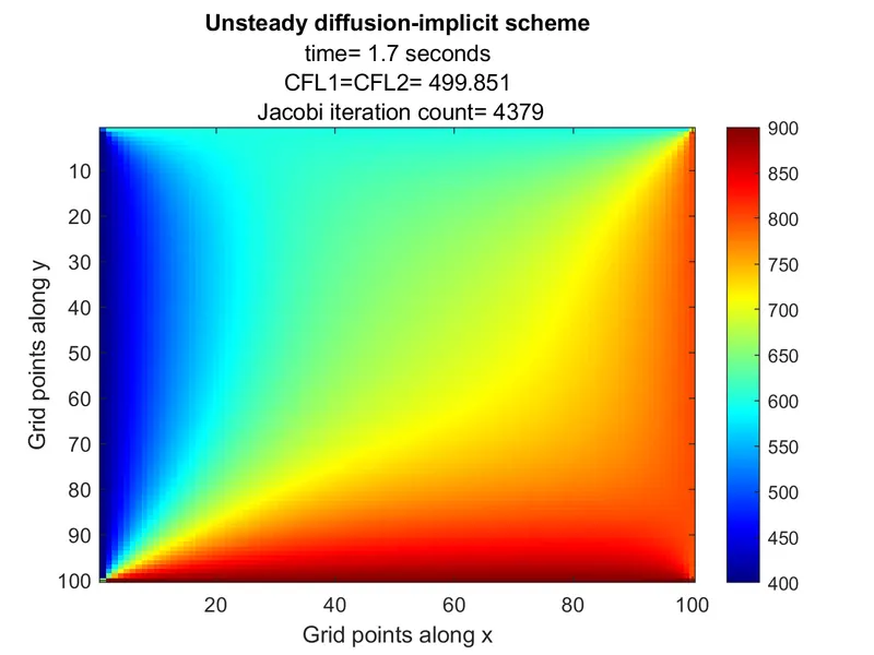
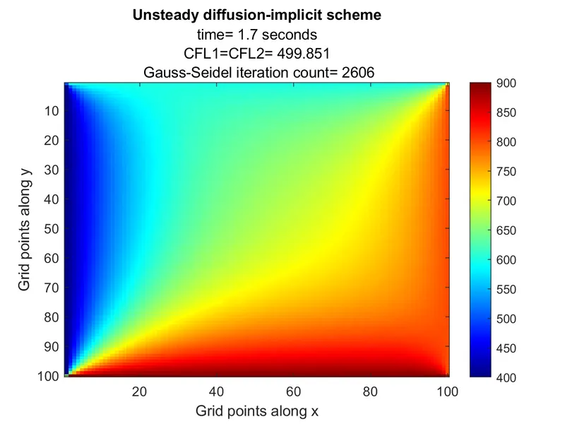
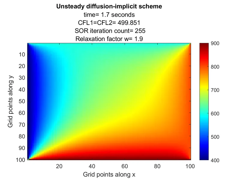
end
Outputs:
Conclusions and Observations:
- It is found that for the given grid size Relaxation factor w=1.9, requires least number of iterations in order to converge to the required tolerance. The order of iteration count for the given grid size, and the error tolerance is found to be Successive Over Relaxation (SOR) < Gauss-Seidel < Jacobi for implict and steady state solution.
- The overall CFL number (CFL1+CFL2) in the explicit case is maintained at 0.49372 . However, implicit scheme has no effect of CFL number(CFL=499.851) and exhibits unconditional stability.
- The explicit scheme is much faster in code performance and easier to formulate as compared to implicit scheme.