Week 3.5 - Deriving 4th order approximation of a 2nd order derivative using Taylor Table method
The Taylor series expressions required to derive the 4th order accurate schemes are :
`f(x+Deltax)=f(x)+f'(x)Deltax+f''(x)(Deltax)^2/(2!)+f'''(x)(Deltax)^3/(3!)+f''''(x)(Deltax)^4/(4!)`
`f(x+2Deltax)=f(x)+f'(x)2Deltax+f''(x)(2Deltax)^2/(2!)+f'''(x)(2Deltax)^3/(3!)+f''''(x)(2Deltax)^4/(4!)`
`f(x-Deltax)=f(x)-f'(x)Deltax+f''(x)(Deltax)^2/(2!)-f'''(x)(Deltax)^3/(3!)+f''''(x)(Deltax)^4/(4!)`
`f(x-2Deltax)=f(x)-f'(x)2Deltax+f''(x)(2Deltax)^2/(2!)-f'''(x)(2Deltax)^3/(3!)+f''''(x)(2Deltax)^4/(4!)` and others.
The Taylor table for Central Difference scheme :
| `f(x)` | `f'(x)Deltax` | `f''(x)(Deltax)^2` | `f'''(x)(Deltax)^3` | `f''''(x)(Deltax)^4` | `f^(v)(x)(Deltax)^5` | `f^(vi)(x)(Deltax)^6` | |
| `A f(x-2Deltax)` | A | -2A | (4/2)A | -(8/6)A | (16/24)A | -(32/120)A | (64/720)A |
| `Bf(x-Deltax)` | B | -B | (1/2)B | -(1/6)B | (1/24)B | -(1/120)B | (1/720)B |
| `Cf(x)` | C | 0 | 0 | 0 | 0 | 0 | 0 |
| `Df(x+Deltax)` | D | D | (1/2)D | (1/6)D | (1/24)D | (1/120)D | (1/720)D |
| `Ef(x+2Deltax)` | E | 2E | (4/2)E | (8/6)E | (16/24)E | (32/120)E | (64/720)E |
| Resulting Co-efficients | 0 | 0 | 1 | 0 | 0 | ----- | ------ |
where A,B,C,D,E are the co-efficients multiplied to each of the taylor expressions, the co-efficients are summed and equated to 0 or 1 (if that term is required it is equated to 1 else to 0).
Re-writing the table in the form of system of equations.
`A+B+C+D+E=0`
`-2A-B+D+2E=0`
`(4/2)A+(1/2)B+(1/2)D+(4/2)E=1`
`-(8/6)A-(1/6)B+(1/6)D+(8/6)E=0`
`(16/24)A+(1/24)B+(1/24)D+(16/24)E=0`
Converting system of equations to matrix representation.
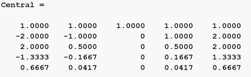
`[[1,1,1,1,1],[-2,-1,0,1,2],[4/2,1/2,0,1/2,4/2],[-8/6,-1/6,0,1/6,8/6],[16/24,1/24,0,1/24,16/24]]` `[[A],[B],[C],[D],[E]]`=`[[0],[0],[1],[0],[0]]`
Code:
% Co-efficient matrix of Central difference scheme
Central=[[1,1,1,1,1];[-2,-1,0,1,2];[4/2,1/2,0,1/2,4/2];[-8/6,-1/6,0,1/6,8/6];[16/24,1/24,0,1/24,16/24]]
Output:
Code:
% Values of unknown co-efficients
XC=inv(Central)*[0 0 1 0 0]'
Output:
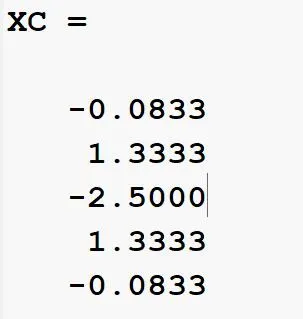
`[[A],[B],[C],[D],[E]]`=`[[-1/12 ],[4/3] , [ -5/2] , [ 4/3] ,[ -1/12 ]]`=`[[-1/12 ],[16/12] , [ -30/12] , [ 16/12] ,[ -1/12 ]]`
The expression reduces to
`f''(x)+f^(vi)(x)(Deltax)^4/270=(-f(x-2Deltax)+16f(x-Deltax)-30f(x)+16f(x+Deltax)-f(x+2Deltax))/(12(Deltax)^2)`
`f^v(x)` term gets cancelled due to symmetry of co-efficients.
`f''(x)+O(Deltax)^4=(-f(x-2Deltax)+16f(x-Deltax)-30f(x)+16f(x+Deltax)-f(x+2Deltax))/(12(Deltax)^2)`
By truncating we get fourth order approximate scheme.
`f''(x)~~(-f(x-2Deltax)+16f(x-Deltax)-30f(x)+16f(x+Deltax)-f(x+2Deltax))/(12(Deltax)^2)`
The Taylor table for Forward Skewed Scheme :
| `f(x)` | `f'(x)Deltax` | `f''(x)(Deltax)^2` | `f'''(x)(Deltax)^3` | `f''''(x)(Deltax)^4` | `f^(v)(x)(Deltax)^5` | `f^(vi)(x)(Deltax)^6` | |
| `A f(x)` | A | 0 | 0 | 0 | 0 | 0 | 0 |
| `Bf(x+Deltax)` | B | B | (1/2)B | (1/6)B | (1/24)B | (1/120)B | (1/720)B |
| `Cf(x+2Deltax)` | C | 2C | (4/2)C | (8/6)C | (16/24)C | (32/120)C | (64/720)C |
| `Df(x+3Deltax)` | D | 3D | (9/2)D | (27/6)D | (81/24)D | (243/120)D | (729/720)D |
| `Ef(x+4Deltax)` | E | 4E | (16/2)E | (64/6)E | (256/24)E | (1024/120)E | (4096/720)E |
| `Ff(x+5Deltax)` | F | 5F | (25/2)F | (125/6)F | (625/24)F | (3125/120)F | (6250/720)F |
| Resulting Co-efficients | 0 | 0 | 1 | 0 | 0 | 0 |
------ |
where A,B,C,D,E are the co-efficients multiplied to each of the taylor expressions in order to cancel out unneccessary terms.
Re-writing the table in the form of system of equations.
`A+B+C+D+E+F=0`
`B+2C+3D+4E+5F=0`
`(1/2)B+(4/2)C+(9/2)D+(16/2)E+(25/2)F=1`
`(1/6)B+(8/6)C+(27/6)D+(64/6)E+(125/6)F=0`
`(1/24)B+(16/24)C+(81/24)D+(256/24)E+(625/24)F=0`
`(1/120)B+(32/120)C+(243/120)D+(1024/120)E+(3125/120)F=0`
Converting system of equations to matrix representation
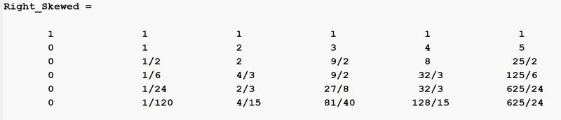
`[[1,1,1,1,1,1],[0,1,2,3,4,5],[0,1/2,4/2,9/2,16/2,25/2],[0,1/6,8/6,27/6,64/6,125/6],[0,1/24,16/24,81/24,256/24,625/24],[0,1/120,32/120,243/120,1024/120,3125/120]]` `[[A],[B],[C],[D],[E],[F]]`=`[[0],[0],[1],[0],[0],[0]]`
Code:
% Co-efficient matrix of Right skewed scheme
Right_Skewed=[[1,1,1,1,1,1];[0,1,2,3,4,5];[0,1/2,4/2,9/2,16/2,25/2];[0,1/6,8/6,27/6,64/6,125/6];[0,1/24,16/24,81/24,256/24,625/24];[0,1/120,32/120,243/120,1024/120,3125/120]]
Output:
On solving,
Code:
% To find the unknown co-efficients
XR=inv(Right_Skewed)*[0 0 1 0 0 0]'
Output:
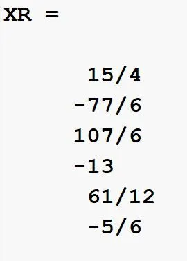
`[[A],[B],[C],[D],[E],[F]]=[[15/4], [-77/6] , [107/6] , [ -13] , [ 61/12] , [-5/6 ]] =[[45/12],[-154/12],[214/12],[-156/12],[61/12],[-10/12]]`
The expression reduces to
`f''(x)+f^(vi)(x)*4843(Deltax)^4/480=(45f(x)-154f(x+Deltax)+214f(x+2Deltax)-156f(x+3Deltax)+61f(x+4Deltax)-10f(x+5Deltax))/(12(Deltax)^2)`
`f''(x)+O(Deltax)^4=(45f(x)-154f(x+Deltax)+214f(x+2Deltax)-156f(x+3Deltax)+61f(x+4Deltax)-10f(x+5Deltax))/(12(Deltax)^2)`
The Taylor table for Backward Skewed Scheme :
| `f(x)` | `f'(x)Deltax` | `f''(x)(Deltax)^2` | `f'''(x)(Deltax)^3` | `f''''(x)(Deltax)^4` | `f^(v)(x)(Deltax)^5` | f^(vi)(x)(Deltax)^6 | |
| `A f(x)` | A | 0 | 0 | 0 | 0 | 0 | |
| `Bf(x-Deltax)` | B | -B | (1/2)B | - (1/6)B | (1/24)B | -(1/120)B | (1/720)B |
| `Cf(x-2Deltax)` | C | -2C | (4/2)C | -(8/6)C | (16/24)C | -(32/120)C | (64/720)C |
| `Df(x-3Deltax)` | D | -3D | (9/2)D | -(27/6)D | (81/24)D | -(243/120)D | (729/720)D |
| `Ef(x-4Deltax)` | E | -4E | (16/2)E | -(64/6)E | (256/24)E | -(1024/120)E | (4096/720)E |
| `Ff(x-5Deltax)` | F | -5F | (25/2)F | -(125/6)F | (625/24)F | -(3125/120)F | (6250/720)F |
| Resulting Co-efficients | 0 | 0 | 1 | 0 | 0 | 0 |
----------- |
where A,B,C,D,E are the co-efficients multiplied to each of the taylor expressions in order to cancel out unneccessary terms.
Re-writing the table in the form of system of equations.
`A+B+C+D+E+F=0`
`-B-2C-3D-4E-5F=0`
`(1/2)B+(4/2)C+(9/2)D+(16/2)E+(25/2)F=1`
`-(1/6)B-(8/6)C-(27/6)D-(64/6)E-(125/6)F=0`
`(1/24)B+(16/24)C+(81/24)D+(256/24)E+(625/24)F=0`
`-(1/120)B-(32/120)C-(243/120)D-(1024/120)E-(3125/120)F=0`
Converting system of equations to matrix representation.
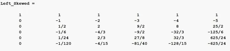
`[[1,1,1,1,1,1],[0,-1,-2,-3,-4,-5],[0,1/2,4/2,9/2,16/2,25/2],[0,-1/6,-8/6,-27/6,-64/6,-125/6],[0,1/24,16/24,81/24,256/24,625/24],[0,-1/120,-32/120,-243/120,-1024/120,-3125/120]]``[[A],[B],[C],[D],[E],[F]]`=`[[0],[0],[1],[0],[0],[0]]`
Code:
% Co-efficient matrix of Left Skewed scheme
Left_Skewed=[[1,1,1,1,1,1];[0,-1,-2,-3,-4,-5];[0,1/2,4/2,9/2,16/2,25/2];[0,-1/6,-8/6,-27/6,-64/6,-125/6];[0,1/24,16/24,81/24,256/24,625/24];[0,-1/120,-32/120,-243/120,-1024/120,-3125/120]]
Output:
Code:
% To find the unknown co-efficients
XL=inv(Left_Skewed)*[0 0 1 0 0 0]'
Output:
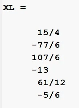
`[[A],[B],[C],[D],[E],[F]]=[[15/4], [-77/6] , [107/6] , [ -13] , [ 61/12] , [-5/6 ]] =[[45/12],[-154/12],[214/12],[-156/12],[61/12],[-10/12]]`
The expression reduces to
`f''(x)+f^(vi)(x)*4843(Deltax)^4/480=(45f(x)-154f(x-Deltax)+214f(x-2Deltax)-156f(x-3Deltax)+61f(x-4Deltax)-10f(x-5Deltax))/(12(Deltax)^2)`
`f''(x)+O(Deltax)^4=(45f(x)-154f(x-Deltax)+214f(x-2Deltax)-156f(x-3Deltax)+61f(x-4Deltax)-10f(x-5Deltax))/(12(Deltax)^2)`
Code:
% Value of x at which the Derivative should be evaluated
x=pi/3;
% Values of dx
dx=linspace(pi/10,pi/800,100);
% Function f(x)
fx=exp(x)*cos(x);
% Analytical Derivative
dfx=-2*exp(x)*sin(x);
% Fourth order Central Difference scheme for the above function
fcdx=(-(exp(x-2*dx).*cos(x-2*dx))+(16*(exp(x-dx).*cos(x-dx)))-(30*fx)+(16*(exp(x+dx).*cos(x+dx)))-(exp(x+2.*dx).*cos(x+2*dx)))./((12*dx.^2));
% Fourth order Forward Difference scheme for the above function
ffdx=(45*fx-154*(exp(x+dx).*cos(x+dx))+214*(exp(x+2*dx).*cos(x+2*dx))-156*(exp(x+3*dx).*cos(x+3*dx))+61*(exp(x+4*dx).*cos(x+4*dx))-10*(exp(x+5*dx).*cos(x+5*dx)))./(12*dx.^2);
% Fourth order Backward Difference scheme for the above function
fbdx=(45*fx-154*(exp(x-dx).*cos(x-dx))+214*(exp(x-2*dx).*cos(x-2*dx))-156*(exp(x-3*dx).*cos(x-3*dx))+61*(exp(x-4*dx).*cos(x-4*dx))-10*(exp(x-5*dx).*cos(x-5*dx)))./(12*dx.^2);
% Error
EC=abs(dfx-fcdx); % Central Differencing
EF=abs(dfx-ffdx); % Forward Differencing
EB=abs(dfx-fbdx); % Backward Differencing
% Error plot
semilogy(dx,EC)   % plotting on dx on linear scale and Error on semilog scale
hold on
semilogy(dx,EF)   % plotting on dx on linear scale and Error on semilog scale
hold on
semilogy(dx,EB)   % plotting on dx on linear scale and Error on semilog scale
xlabel('dx')      % label x axis as dx
ylabel('Absolute Error') % label y axis as Absolute error
legend('Central Difference','Forward Difference','Backward Difference') % Defining legends
Outputs:
Conclusions:
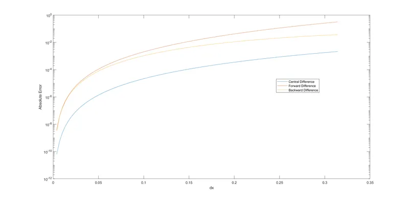
- From the graph it is clear that Central Difference Scheme is the most accurate scheme among Backward and Forward Differencing. The order of accuracy Central Differencing scheme> Backward Differencing scheme >Forward Differencing scheme for their respective grid sizes.
- The skewed schemes are required when there are no nodes on one side. Example, at boundaries the domain might exist only in certain directions, there the skewed schemes are required due to non-existence of the domain in a direction.