Week 5.1 - Mid term project - Solving the steady and unsteady 2D heat conduction problem
The 2D heat conduction equation is of 2 types:
1) steady-state
2) unsteady-state
The steady-state equation can be solved with the implicit method while coming to the unsteady state equation there is a time term, so it can be solved either explicit or implicit method.
For steady-state eq
((del^2T)/(delx^2)+(del^2T)/(dely^2)) = 0`
where T is temperature and x,y are special coordinates.
T_p= 1/k*((T_l+T_r)/(Deltax^2)) + 1/k*((T_t+T_b)/(Deltay^2))`
If the above equation in nodes(i,j) form, then the equation should be
T(i,j) = 1/k*((T_(i-1,j)+T_(i+1,j))/(Deltax^2)) + 1/k*((T_(i,j-1)+T_(i,j+1))/(Deltay^2))`
steady-state equation:
function code:
for the Jacobi
function out = jacob_1(t,told,i,j)
out = 0.25*((told(i,j-1)+told(i,j+1)+told(i-1,j)+told(i+1,j)))
end
for the GS
function out = GS_1(t,told,i,j)
out = 0.25*((t(i,j-1)+told(i,j+1)+t(i-1,j)+told(i+1,j)))
end
for the Sor
function out = sor_1(t,told,i,j,f)
out = (1-f)*told(i,j) + f*(0.25*(t(i,j-1)+told(i,j+1)+t(i-1,j)+told(i+1,j)))
end
main code:
clear all
close all
clc
% inputs
% number of grid points along x and y axis
nx= 10;
ny=10;
x=linspace(0,1,nx);
dx = x(2)-x(1);
y= linspace(0,1,ny);
z=fliplr(y);
f=1.1;
iter = 1;
t= 300*ones([nx,ny]);
% applying BC
t(1,:)=600;
t(end,:)=900;
t(:,1)=400;
t(:,end)=800;
% creating a copy
told=t;
r1=t;
error= 19;
tol = 1e-4;
for iterative_solver = 1:3;
while(error>tol);
for i=2:nx-1;
for j=2:ny-1;
if(iterative_solver==1);
t(i,j)= jacob_1(t,told,i,j);
elseif(iterative_solver==2)
t(i,j)=GS_1(t,told,i,j);
elseif(iterative_solver==3)
t(i,j)= sor_1(t,told,i,j,f);
end
end
end
error = max(max(t-told));
told = t;
[u1,v1]=meshgrid(x,z);
% plot
if(iterative_solver==1);
figure(1);
contourf(u1,v1,t);
[C,h]= contourf(u1,v1,t);
colorbar;
colormap(jet);
clabel(C,h);
xlabel('x-axis');
ylabel('y-axis');
title_text=sprintf('jacobi iterantion number=%d',iter);
title(title_text);
pause(0.003);
elseif(iterative_solver==2);
figure(2);
contourf(u1,v1,t);
[C,h]= contourf(u1,v1,t);
colorbar;
colormap(jet);
clabel(C,h);
xlabel('x-axis');
ylabel('y-axis');
title_text=sprintf('GS iterantion number=%d',iter);
title(title_text);
pause(0.003);
else
figure(3);
[C,h]= contourf(u1,v1,t);
colorbar;
colormap(jet);
clabel(C,h);
xlabel('x-axis');
ylabel('y-axis');
title_text=sprintf('sor iterantion number=%d',iter);
title(title_text);
pause(0.003);
end
iter=iter+1;
end
error=19;
iter=1;
t=r1;
told=t;
end
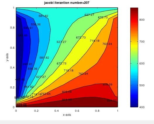
For Jacobi
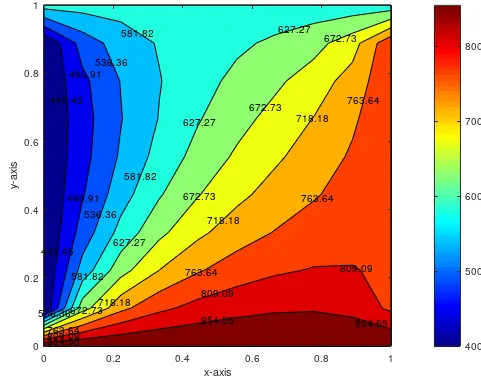
For GS
for SOR
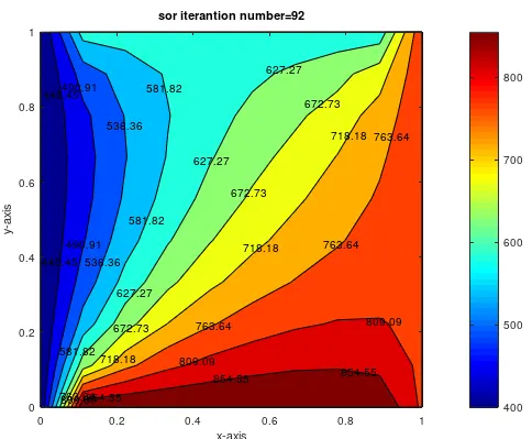
From the above, we can conclude that the s o r method is the fastest method as it solves the equation in 92 iterations.
For unsteady
`(delT)/(delt)= alpha*((del^2T)/(delx^2)+(del^2T)/(dely^2))`,
where T is time and x,y are special coordinates.
As mentioned before, the unsteady state equation solved in 2 methods. They are Explicit and Implicit methods.
For Explicit method:
The equation in terms of nodes(i,j)
`T_p^(n+1)= T_p^n+k1*(T_l-2*T_p+T_r)^n + k2*(T_t-2*T_p+T_b)^n`
where `K_1 = alpha*(trianglet)/(trianglex^2)`, `K_2 = alpha*(trianglet)/(triangley^2)`
If `K_1 + K_2` is greater than 0.5 then it is a unsteable.
For Implicit method:
The equation in terms of nodes(i,j)
`T_p^(n+1)= Term1*(T_p^n+k_1*(T_l+T_r)^(n+1) + k_2*(T_t+T_b)^(n+1))`
where term1 = 1/(1+2*k_1+2*k_2), term2 = `K_1`*term1, term3 = `K_2`*term1
code for Transient method:
Explicit method:
clear all
close all
clc
% inputs
% number of grid points along x and y axis
nx= 10;
ny=10;
x=linspace(0,1,nx);
dx = x(2)-x(1);
y= linspace(0,1,ny);
dy = y(2)-y(1);
c= 1;
% number of steps
nt=200;
% time steps
dt = 0.001;
% CFL number
k= (c*dt)/dx^2;
t= ones([nx,ny])*673;
% applying BC
t(1,:)=600;
t(end,:)=900;
t(:,1)=400;
t(:,end)=800;
told = t;
tic
iter=1
for p=1:nt
for i= 2:nx-1
for j=2:ny-1
t(i,j)= k*(told(i-1,j)+told(i+1,j)+told(i,j+1)+told(i,j-1))+ (1-4*k)*told(i,j);
endfor
error=max(abs(told-t));
told=t;
iter=iter+1;
endfor
time = toc;
figure(1)
[c,h]=contourf(x,fliplr(y),t);
colorbar;
colormap(jet);
clabel(c,h);
title(sprintf('2D unsteady heat conduction (Explicit method) n iteration number=%d; t computational time :%0.4f',iter,time));
xlabel('xx');
ylabel('yy');
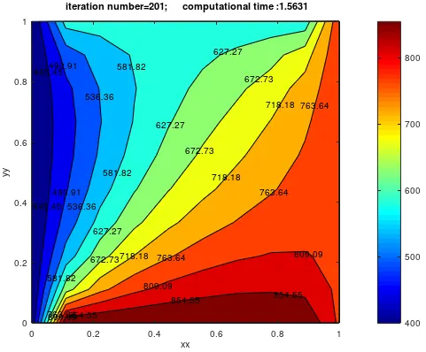
for explicit :
code for Implicit method:
clear all
close all
clc
% inputs
% number of grid points along x and y axis
nx= 10;
ny=10;
x=linspace(0,1,nx);
dx = x(2)-x(1);
y= linspace(0,1,ny);
dy = y(2)-y(1);
f= 1.2;
t= ones(nx,ny)*298;
% applying BC
t(1,:)=600;
t(end,:)=900;
t(:,1)=400;
t(:,end)=800;
alpha= 1.4;
dt=0.001;
% defining k1 and k2
k1=alpha*(dt/dx^2);
k2=alpha*(dt/dy^2);
told=t;
t_initial=t;
for iterartive_solver = 1:3
nt=1:1400;
error=9e9;
tol=1;
tic;
% iterartive_solver==1:3;
iter=1;
while error>tol
for i=2:nx-1
for j=2:ny-1
term1= 1/(1+2*k1+2*k2);
term2= k1*term1;
term3= k2*term1;
if iterartive_solver==1;
t(i,j)= ((told(i,j)*term1)+(term2*(t(i-1,j)+t(i+1,j))+(term3*(t(i,j-1)+t(i,j+1)))));
elseif iterartive_solver==2;
t(i,j)= ((told(i,j)*term1)+(term2*(t(i-1,j)+told(i+1,j))+(term3*(t(i,j-1)+told(i,j+1)))));
elseif iterartive_solver==3;
t(i,j)= (1-f)*told(i,j)+ f*(((told(i,j)*term1)+(term2*(t(i-1,j)+told(i+1,j))+(term3*(t(i,j-1)+told(i,j+1))))));
end
end
error_n=max(abs(told-t));
error=max(error_n);
told=t;
iter=iter+1;
end
end
time=toc;
%plot
if iterartive_solver==1;
figure(1)
contourf(x,fliplr(y),t);
[C,h]=contourf(x,fliplr(y),t);
colorbar;
colormap(jet);
clabel(C,h);
text = sprintf('JACOBI Method n iteration number = %d; t computational time: %0.4f',iter ,time);
title(text);
told=t_initial;
t=t_initial;
elseif iterartive_solver==2;
figure(2)
[c,h]=contourf(x,fliplr(y),t);
colorbar;
colormap(jet);
clabel(c,h);
title(sprintf('GS Method n iteration number = %d; t computational time: %0.4f',iter,time));
told=t_initial;
t=t_initial;
else
figure(3)
[c,h]=contourf(x,fliplr(y),t);
colorbar;
colormap(jet);
clabel(c,h);
title(sprintf('SOR Method n iteration number = %d; t computational time: %0.4f',iter,time));
told=t_initial;
t=t_initial;
end
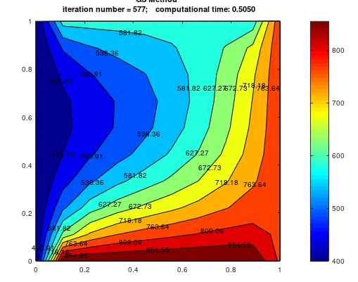
GS
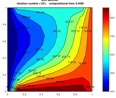
sor
observation and results :
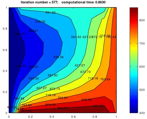
the Implicit method is more accurate as it uses various iterative solvers.From the above plots, it can be found that the explicit scheme is the fastest to solve the transient 2D heat equation as we are not bothered about iteration and convergence.
The advantage of an Explicit scheme is that it doesn't need guess value and convergence criteria.
But the explicit scheme has to be strictly governed by CFL stability condition
i.e `CFL <= 0.5`to offer better stability .
If we see the Implicit Scheme are slower and more complicated than the explicit scheme since we are using guess value and iteration for convergence at each time step
However, they are unconditionally stable for any choice with respect to dx.
In the implicit plot, we notice that the Jacobi method took the most number of iteration to converge followed by SOR(omega =1.5) and then Gauss Seidel.
In the steady-state method, there is no time loop and the results converge within we iterations.
Whereas in the implicit method, the introduction of time loop results converges to run with a large number of iterations.
Computation time is more for transient solver as it is a function of both time and position.
Whereas, in the case of a steady-state solver, it's a function of the only position.
Successive Over Relaxation method converges with less number of iteration and computational time.
While comparing both Explicit and Implicit methods results, the Explicit method is much quicker than the implicit method. The Explicit method takes 201 iterations whereas the Implicit method takes 577, 577, 521 iterations. Coming to the implicit method SOR is the fastest method while comparing it with Jacobi and GS. The SOR method took 521 iterations, the Implicit method is more accurate as it uses various iterative solvers.