Week 5.1 - Mid term project - Solving the steady and unsteady 2D heat conduction problem
Objective - To solve the steady and unsteady 2D heat conduction equation ny using the iterative techniques such as jacobi, Gauss-seidel & Successive over relaxation for both implicit and explicit schemes using MATLAB.
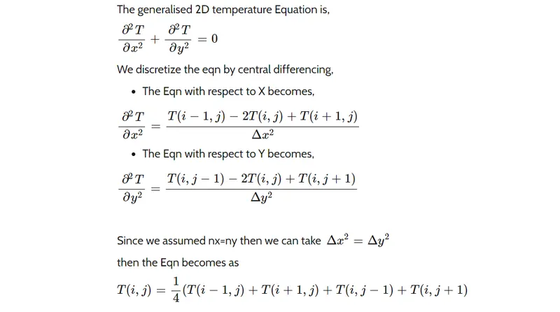
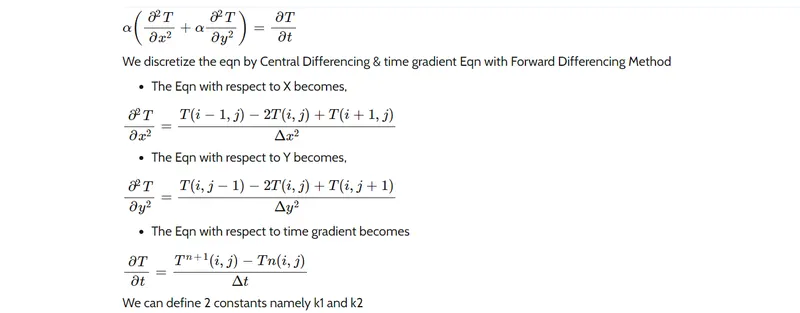
2D heat conduction equation is given by,
∂T/∂t = alpha* ( ∂2T/∂x2 + ∂2T/∂x2)
Theoretical part -
transfer of energy may occure under two conditions.
1) Steady state condition-
A flui state in which there is no change in the fluid property w.r.t to time is called steady state. The fluid property is temperature, so
MATLAB program -
Using Jacobi method,
clear all
close all
clc

%steady state 2nd order heat conduction eqn(2D)
%inputs
l=1;
nx=10;
ny=nx;
dx=l/(nx-1);
dy=l/(ny-1);
x=linspace(0,1,nx);
y=linspace(0,1,ny);

%temperatures given
T_l=400;
T_t=600;
T_r=800;
T_b=900;
T=ones(nx,ny);

%updating values of temperatures
T(:,1)=T_l;
T(:,end)=T_r;
T(1,:)=T_t;
T(end,:)=T_b;
Told=T;
[X Y]=meshgrid(x,y);


iterative_solver=1;
error=9e9;
tol=1e-4;

%jacobi method
tic;
jacobi_iter=1;
while(error>tol)
    for i=2:nx-1
        for j=2:ny-1
            T(i,j)=0.25*((Told(i-1,j)+Told(i+1,j)))+0.25*((Told(i,j-1)+Told(i,j+1)));
        end
    end
    error=max(max(abs(Told-T)));
    Told=T;
    jacobi_iter=jacobi_iter+1;
end

A=toc;

figure(1)
contourf(X,Y,T,'showtext','on')
colormap(jet);
colorbar;
title_text=sprintf('jacobi,iterations=%d,simulation time=%f',jacobi_iter,A);
title(title_text);
xlabel('x axis');
ylabel('y axis');
pause(0.003);
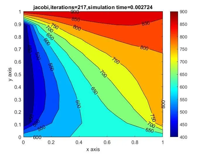
Temperature field plot -
Using Gauss seidel method,
clear all
close all
clc

%steady state 2nd order heat conduction eqn(2D)
%inputs
l=1;
nx=10;
ny=nx;
dx=l/(nx-1);
dy=l/(ny-1);
x=linspace(0,1,nx);
y=linspace(0,1,ny);

%temperatures given
T_l=400;
T_t=600;
T_r=800;
T_b=900;
T=ones(nx,ny);

%updating values of temperatures
T(:,1)=T_l;
T(:,end)=T_r;
T(1,:)=T_t;
T(end,:)=T_b;
Told=T;
[X Y]=meshgrid(x,y);


iterative_solver=1;
error=9e9;
tol=1e-4;

%GS method
tic;
gs_iter=1;
while(error>tol)
    for i=2:nx-1
        for j=2:ny-1
            T(i,j)=0.25*((T(i-1,j)+Told(i+1,j)))+0.25*((T(i,j-1)+Told(i,j+1)));
        end
    end
    error=max(max(abs(Told-T)));
    Told=T;
    gs_iter=gs_iter+1;
end

B=toc;

figure(2)
contourf(X,Y,T,'showtext','on')
colormap(jet);
colorbar;
title_text=sprintf('gs,iterations=%d,simulation time=%f',gs_iter,B);
title(title_text);
xlabel('x axis');
ylabel('y axis');
pause(0.003);
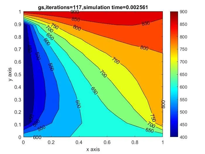
Plot -
Using SOR method,
clear all
close all
clc

%steady state 2nd order heat conduction eqn(2D)
%inputs
l=1;
nx=10;
ny=nx;
dx=l/(nx-1);
dy=l/(ny-1);
x=linspace(0,1,nx);
y=linspace(0,1,ny);

%temperatures given
T_l=400;
T_t=600;
T_r=800;
T_b=900;
T=ones(nx,ny);

%updating values of temperatures
T(:,1)=T_l;
T(:,end)=T_r;
T(1,:)=T_t;
T(end,:)=T_b;
Told=T;
[X Y]=meshgrid(x,y);


iterative_solver=1;
error=9e9;
tol=1e-4;

%SOR method
tic;
sor_iter=1;
omega=1.1;
while(error>tol)
    for i=2:nx-1
        for j=2:ny-1
            T(i,j)=(1-omega)*Told(i,j)+omega*(0.25*((T(i-1,j)+Told(i+1,j)))+0.25*((T(i,j-1)+Told(i,j+1))));
        end
    end
    error=max(max(abs(Told-T)));
    Told=T;
    sor_iter=sor_iter+1;
end

C=toc;

figure(3)
contourf(X,Y,T,'showtext','on')
colormap(jet);
colorbar;
title_text=sprintf('sor,iterations=%d,simulation time=%f',sor_iter,C);
title(title_text);
xlabel('x axis');
ylabel('y axis');
pause(0.003);
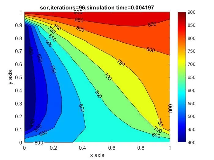
Plot -
2) Unsteady state condition

Solving Transient state explicitly -
clear all
close all
clc

%transient state 2nd order heat conduction eqn(2D)explicitly
%inputs
l=1;
nx=10;
ny=nx;
dx=l/(nx-1);
dy=l/(ny-1);
alpha=1.4;
dt=0.001;
t=0.2;
nt=t/dt;
x=linspace(0,1,nx);
y=linspace(0,1,ny);

%temperatures given
T_l=400;
T_t=600;
T_r=800;
T_b=900;
T=ones(nx,ny);

%updating values of temperatures
T(:,1)=T_l;
T(:,end)=T_r;
T(1,:)=T_t;
T(end,:)=T_b;
Told=T;
[X Y]=meshgrid(x,y);


iterative_solver=1;
error=9e9;
tol=1e-4;
alpha=1.4;

%CFL number calculation
k1=(alpha*dt)/dx^2;
k2=(alpha*dt)/dy^2;


%explicitly solving
tic;
explicit_iter=1;
while(error>tol)
    for k=1:nt;
    for i=2:nx-1
        for j=2:ny-1
            T(i,j)=Told(i,j)+k1*(Told(i-1,j)-2*Told(i,j)+Told(i+1,j))+k2*(Told(i,j-1)-2*Told(i,j)+Told(i,j+1));
        end
    end
    error=max(abs(Told-T));
    Told=T;
    explicit_iter=explicit_iter+1;
    end

end

time=toc;

figure(1)
contourf(X,Y,T,'showtext','on')
colormap(jet);
colorbar;
title_text=sprintf('explicit,iterations=%d,simulation time=%f',explicit_iter,time);
title(title_text);
xlabel('x axis');
ylabel('y axis');
pause(0.003);
Solving transient state implicitly -
1) jacobi method
clear all
close all
clc

%transient state 2nd order heat conduction eqn(2D)implicitly
%inputs
l=1;
nx=10;
ny=nx;
dx=l/(nx-1);
dy=l/(ny-1);
alpha=1.4;
dt=1;
t=5;
nt=t/dt;
cfl=(alpha*dt)/dx^2;
x=linspace(0,1,nx);
y=linspace(0,1,ny);

%temperatures given
T_l=400;
T_t=600;
T_r=800;
T_b=900;
T=ones(nx,ny);

%updating values of temperatures
T(:,1)=T_l;
T(:,end)=T_r;
T(1,:)=T_t;
T(end,:)=T_b;
Told=T;
T_previous=T;
[X Y]=meshgrid(x,y);


iterative_solver=1;
error=9e9;
tol=1e-4;
alpha=1.4;

%CFL number calculation
k1=(alpha*dt)/dx^2;
k2=(alpha*dt)/dy^2;

term1=(1+2*k1+2*k2)^-1;
term2=k1*term1;
term3=k2*term1;

%jacobi method
tic;
jacobi_iter=1;
for k=1:nt

    while(error>tol)

    for i=2:nx-1
        for j=2:ny-1
            H=(Told(i-1,j)+Told(i+1,j));
            V=(Told(i,j-1)+Told(i,j+1));
            T(i,j)=(term1*T_previous(i,j))+(term2*H)+(term3*V);
        end
    end
    error=max(max(abs(Told-T)));
    Told=T;
    jacobi_iter=jacobi_iter+1;
    end
    T_previous=T;
end

time=toc;

figure(1)
contourf(X,Y,T,'showtext','on')
colormap(jet);
colorbar;
title_text=sprintf('jacobi,iterations=%d,simulation time=%f',jacobi_iter,time);
title(title_text);
xlabel('x axis');
ylabel('y axis');
pause(0.003);
2) Gauss seidel method
clear all
close all
clc

%transient state 2nd order heat conduction eqn(2D)implicitly
%inputs
l=1;
nx=10;
ny=nx;
dx=l/(nx-1);
dy=l/(ny-1);
alpha=1.4;
dt=1;
t=5;
nt=t/dt;
cfl=(alpha*dt)/dx^2;
x=linspace(0,1,nx);
y=linspace(0,1,ny);

%temperatures given
T_l=400;
T_t=600;
T_r=800;
T_b=900;
T=ones(nx,ny);

%updating values of temperatures
T(:,1)=T_l;
T(:,end)=T_r;
T(1,:)=T_t;
T(end,:)=T_b;
Told=T;
T_previous=T;
[X Y]=meshgrid(x,y);


iterative_solver=1;
error=9e9;
tol=1e-4;
alpha=1.4;

%CFL number calculation
k1=(alpha*dt)/dx^2;
k2=(alpha*dt)/dy^2;

term1=(1+2*k1+2*k2)^-1;
term2=k1*term1;
term3=k2*term1;

%GS method
tic;
gs_iter=1;
for k=1:nt

    while(error>tol)

    for i=2:nx-1
        for j=2:ny-1
            H=(T(i-1,j)+Told(i+1,j));
            V=(T(i,j-1)+Told(i,j+1));
            T(i,j)=(term1*T_previous(i,j))+(term2*H)+(term3*V);
        end
    end
    error=max(max(abs(Told-T)));
    Told=T;
    gs_iter=gs_iter+1;
    end
    T_previous=T;
end

time=toc;

figure(2)
contourf(X,Y,T,'showtext','on')
colormap(jet);
colorbar;
title_text=sprintf('gs,iterations=%d,simulation time=%f',gs_iter,time);
title(title_text);
xlabel('x axis');
ylabel('y axis');
pause(0.003);
3) SOR method
clear all
close all
clc

%transient state 2nd order heat conduction eqn(2D)implicitly
%inputs
l=1;
nx=10;
ny=nx;
dx=l/(nx-1);
dy=l/(ny-1);
alpha=1.4;
dt=1;
t=5;
nt=t/dt;
cfl=(alpha*dt)/dx^2;
x=linspace(0,1,nx);
y=linspace(0,1,ny);

%temperatures given
T_l=400;
T_t=600;
T_r=800;
T_b=900;
T=ones(nx,ny);

%updating values of temperatures
T(:,1)=T_l;
T(:,end)=T_r;
T(1,:)=T_t;
T(end,:)=T_b;
Told=T;
T_previous=T;
[X Y]=meshgrid(x,y);


iterative_solver=1;
error=9e9;
tol=1e-4;
alpha=1.4;

%CFL number calculation
k1=(alpha*dt)/dx^2;
k2=(alpha*dt)/dy^2;

term1=(1+2*k1+2*k2)^-1;
term2=k1*term1;
term3=k2*term1;

%SOR method
tic;
omega=1.4;
sor_iter=1;
for k=1:nt;

    while(error>tol)

    for i=2:nx-1
        for j=2:ny-1
            H=(T(i-1,j)+Told(i+1,j));
            V=(T(i,j-1)+Told(i,j+1));
            T(i,j)=((1-omega)*Told(i,j))+omega*((term1*T_previous(i,j))+(term2*H)+(term3*V));
        end
    end
    error=max(max(abs(Told-T)));
    Told=T;
    sor_iter=sor_iter+1;
    end
    T_previous=T;
end

time=toc;

figure(3)
contourf(X,Y,T,'showtext','on')
colormap(jet);
colorbar;
title_text=sprintf('sor,iterations=%d,simulation time=%f',sor_iter,time);
title(title_text);
xlabel('x axis');
ylabel('y axis');
pause(0.003);
Conclusions -
| For steady flow simulation | ||
| Method | Number of iterations | Simulation time |
| Jacobi | 217 | 0.002724 |
| Gauss Seidel | 117 | 0.002561 |
| SOR | 96 | 0.004197 |
| For Unsteady flow simulation | ||
| Method | Number of iterations | Simulation time |
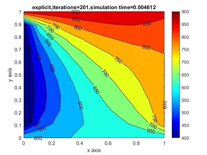
| Explicit scheme | 201 | 0.004612 |
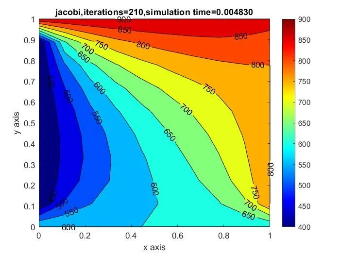
| Jacobi | 210 | 0.00483 |
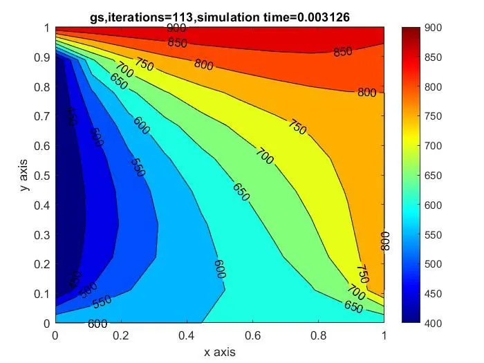
| Gauss Seidel | 113 | 0.003126 |
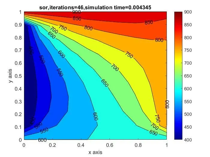
| SOR | 46 | 0.004345 |
From above results, we can affirmly say that Succesive Over Relaxation iterattive method proves to be converging the solution faster and with fewer iterations.