Week 3.5 - Deriving 4th order approximation of a 2nd order derivative using Taylor Table method

Derivation of the 4th order approximations of second order derivative :

P= order of accuracy

Q=order of derivative

N=number of nodes

P=N-Q+1 is the equation for central and symmetrical schemes. That means number of nodes gonna be there are 5.

P=N-Q is the equation for One-sided and skewed schemes. That means number of nodes gonna be there are 6.

Fomulation of taylor method equation for different schemes -

1) Skewed 2nd order right sided difference scheme

2) Skewed 2nd order left sided difference scheme

3) Symmetrical 2nd order central difference scheme

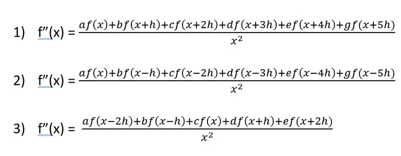
1) Skewed 2nd order right sided difference scheme -

Here we need 6 nodes in order to find the 2nd order derivative with 4th order approximation. Taylor table we get,

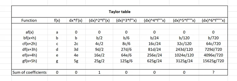
A=[1 1 1 1 1 1;0 1 2 3 4 5;0 1/2 2 9/2 8 25/2;0 1/6 8/6 27/6 64/6 125/6;0 1/24 16/24 81/24 256/24 625/24;0 1/120 32/120 243/120 1024/120 3125/120];
B=[0;0;1;0;0;0];
x_r=inv(A)*B

>> A

A =

    1.0000    1.0000    1.0000    1.0000    1.0000    1.0000
         0    1.0000    2.0000    3.0000    4.0000    5.0000
         0    0.5000    2.0000    4.5000    8.0000   12.5000
         0    0.1667    1.3333    4.5000   10.6667   20.8333
         0    0.0417    0.6667    3.3750   10.6667   26.0417
         0    0.0083    0.2667    2.0250    8.5333   26.0417

>> B

B =

     0
     0
     1
     0
     0
     0

>> x_r

x_r =

    3.7500
  -12.8333
   17.8333
  -13.0000
    5.0833
   -0.8333

>> 

2) Skewed 2nd order left sided difference scheme -

Here we need 6 nodes in order to find the 2nd order derivative with 4th order approximation. Taylor table we get,

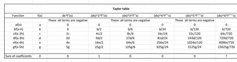
C=[1 1 1 1 1 1;0 -1 -2 -3 -4 -5;0 1/2 2 9/2 8 25/2;0 -1/6 -8/6 -27/6 -64/6 -125/6;0 1/24 16/24 81/24 256/24 625/24;0 -1/120 -32/120 -243/120 -1024/120 -3125/120];
D=[0;0;1;0;0;0];
x_l=inv(C)*D

>> C

C =

    1.0000    1.0000    1.0000    1.0000    1.0000    1.0000
         0   -1.0000   -2.0000   -3.0000   -4.0000   -5.0000
         0    0.5000    2.0000    4.5000    8.0000   12.5000
         0   -0.1667   -1.3333   -4.5000  -10.6667  -20.8333
         0    0.0417    0.6667    3.3750   10.6667   26.0417
         0   -0.0083   -0.2667   -2.0250   -8.5333  -26.0417

>> D

D =

     0
     0
     1
     0
     0
     0

>> x_l

x_l =

    3.7500
  -12.8333
   17.8333
  -13.0000
    5.0833
   -0.8333

>> 

3) Symmetrical 2nd order central difference scheme -

Here we need 5 nodes in order to find the 2nd order derivative with 4th order approximation. Taylor table we get,

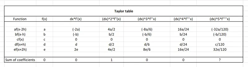
E=[1 1 1 1 1 ;-2 -1 0 1 2 ;2 1/2 0 1/2 2 ;-4/3 -1/6 0 1/6 4/3 ;2/3 1/24 0 1/24 2/3];
F=[0;0;1;0;0];
x_c=inv(E)*F

>> E

E =

    1.0000    1.0000    1.0000    1.0000    1.0000
   -2.0000   -1.0000         0    1.0000    2.0000
    2.0000    0.5000         0    0.5000    2.0000
   -1.3333   -0.1667         0    0.1667    1.3333
    0.6667    0.0417         0    0.0417    0.6667

>> F

F =

     0
     0
     1
     0
     0

>> x_c

x_c =

   -0.0833
    1.3333
   -2.5000
    1.3333
   -0.0833

>> 

Main program:

clear all
close all
clc

x=pi/3;
dx=linspace(pi/4,pi/40,2000);
%Analytical function
%f(x)=exp(x)*cos(x)
%Analytical second order derivative
%f''(x)=-2*exp(x)*sin(x)
analytical_second_order_derivative=-2*exp(x)*sin(x);

A=[1 1 1 1 1 1;0 1 2 3 4 5;0 1/2 2 9/2 8 25/2;0 1/6 8/6 27/6 64/6 125/6;0 1/24 16/24 81/24 256/24 625/24;0 1/120 32/120 243/120 1024/120 3125/120];
B=[0;0;1;0;0;0];
x_r=inv(A)*B;

C=[1 1 1 1 1 1;0 -1 -2 -3 -4 -5;0 1/2 2 9/2 8 25/2;0 -1/6 -8/6 -27/6 -64/6 -125/6;0 1/24 16/24 81/24 256/24 625/24;0 -1/120 -32/120 -243/120 -1024/120 -3125/120];
D=[0;0;1;0;0;0];
x_l=inv(C)*D;


E=[1 1 1 1 1 ;-2 -1 0 1 2 ;2 1/2 0 1/2 2 ;-4/3 -1/6 0 1/6 4/3 ;2/3 1/24 0 1/24 2/3];
F=[0;0;1;0;0];
x_c=inv(E)*F;

%main function
f=@(x)exp(x).*cos(x);

right_skewed_difference=(x_r(1)*f(x)+x_r(2)*f(x+dx)+x_r(3)*f(x+2.*dx)+x_r(4)*f(x+3.*dx)+x_r(5)*f(x+4.*dx)+x_r(6)*f(x+5.*dx))./(dx.^2);
left_skewed_difference=(x_l(1)*f(x)+x_l(2)*f(x-dx)+x_l(3)*f(x-2.*dx)+x_l(4)*f(x-3.*dx)+x_l(5)*f(x-4.*dx)+x_l(6)*f(x-5.*dx))./(dx.^2);
central_difference=(x_c(1)*f(x-2.*dx)+x_c(2)*f(x-dx)+x_c(3)*f(x)+x_c(4)*f(x+dx)+x_c(5)*f(x+2.*dx))./(dx.^2);

error_r=abs(analytical_second_order_derivative-right_skewed_difference);
error_l=abs(analytical_second_order_derivative-left_skewed_difference);
error_c=abs(analytical_second_order_derivative-central_difference);

figure(1)
loglog(dx,error_r)
hold on
loglog(dx,error_l)
loglog(dx,error_c)
xlabel('dx')
ylabel('error')
legend('right skewed difference','left skewed difference','central difference')

Step size input range of (pi/4, pi/40,200) is given.

Plot :

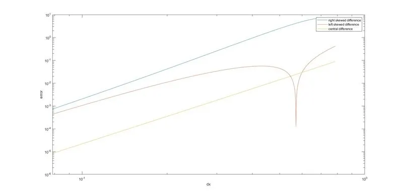
Conclusion :

It is clear from the plot that central difference schemes gives less amount of error compared to other two schemes. But when we have data available that is only from the left and right nodes close to the boundaries, to compute such problems we use skewed schemes.