SIMULATING 2D SUPERSONIC EXPANSION FAN ( PRANDTL MEYER EXPANSION FAN) AND UNDERSTANDING THE EFFECT OF SUB GRID SCALE FACTOR ON SHOCK LOCATION USING CONVERGE CFD

Aim: To simulate the Prandtl Meyer Shock flow in Converge CFD

1. Simulate the supersonic and subsonic flow through a duct having a sharp corner

2. Study the formation of shock waves in the duct

3. Observe the effect of SGS parameter on shock location and cell count.

Introduction and Theory

What is a shock wave?

• The shock wave is produced in an elastic medium when an object moves faster than the local speed of sound. It creates a sudden change in speed, pressure, the temperature of the medium so this can be generated only when the speed of the object reaches above supersonic.
• The generation of shock waves creates a disturbance in the medium with a certain energy and most of it is disputed in the form of heat diffusion.
• In the analysis of a physical model of an object, the generation of the shock wave has treated a loss of energy and it is an irreversible process.
• The model dealing with high velocities should be designed in such a way that there should be a minimum chance for generating a shock wave if it is generated care should be taken such that there should be no damage to the model.

Physics of shocks and expansion fans

A shock wave or shock is a disturbance travelling through a medium at a speed greater than the local speed of sound in that medium. Shocks are accompanied by abrupt changes in pressure, temperature and density of the medium. These changes occur across such small thickness that shocks appear as discontinuities.

In order to understand shocks, let us consider a scenario where an object (source of disturbance) is moving through a quiescent fluid at the local speed of sound in the fluid. The figure shown below displays the spherical wavefronts emanating from the object.

It can be seen that the object keeps up with the spherical wavefronts that it creates since the radius of each spherical wavefront is given by `aDeltat` where `Deltat` is the time elapsed and the distance moved by the source within the same duration is also `aDeltat`.

Let us now consider the scenario where the speed of the object exceeds the local speed of sound in the medium. In other words, the object is moving at supersonic speed.

As shown in the figure, at supersonic speed the spherical wavefronts are unable to keep up with the object (source of disturbance) since within the same time duration `Deltat` the wavefronts travel a distance of `aDeltat` whereas the object moves through a (greater) distance of `vDeltat`. At any time instant the different wavefronts are encompassed by a cone in three dimensions, called the Mach cone. Due to the grouping (constructive interference) of pressure wavefronts at the surface of the cone, shock waves are established. Any region of the fluid which passes through the mach cone, experiences shock and undergoes abrupt changes in pressure, temperature and density.

The half angle `theta` of the mach cone is known as Mach cone angle.

`sin theta=(aDeltat)/(vDeltat)=a/v=1/M` (Mach number)

`theta=arcsin (1/M)`

Like other waves, a shock wave transmits energy through the medium. Across the shock waves, energy is conserved but entropy is created. Hence shocks are highly irreversible processes. The second law of thermodynamics prevents the existence of shocks across which the fluid undergoes expansion. However there are scenarios in which supersonic flows can experience isentropic expansions and compressions. One such scenario where the supersonic flow experiences isentropic expansion at a sharp corner is Prandtl-Meyer expansion fan. Given below is an image showing the Prandtl-Meyer expansion fan.

image taken from https://en.wikipedia.org/wiki/Prandtl%E2%80%93Meyer_expansion_fan

The isentropic expansion experienced by the supersonic flow in Prandtl-Meyer expansion occurs across infinite number of Mach waves (all diverging from the sharp corner), each wave turning the flow by an infinitesimal angle.

Prandtl-Meyer function determines the angle through which a sonic flow (M=1) must turn to reach a particular Mach number (M). Mathematically,

`nu(M)=sqrt((gamma+1)/(gamma-1))arctan (sqrt((gamma+1)/(gamma-1)(M^2-1)))-arctan (sqrt(M^2-1))`

Also the turn angle `theta`is given by

`theta=nu(M_2)-nu(M_1)`

Shock flow boundary conditions-

Neumann Boundary condition is used in this case. “Dirichlet”, “Neumann”, and “Robin” conditions are the three most common boundary conditions used for partial differential equations.

When using a Dirichlet boundary condition, the value of variable is prescribed at the boundary,the value of variable is prescribedat the boundary.

When Neumann boundary conditions imposed on an ordinary or a PDE, the condition specifies the value in which the derivative of a solution is applied within the boundary of domain.

Pressure outlet boundary conditions require the specification of a static pressure at the outlet boundary. The value of the specified static pressure is used only while the flow is subsonic. If the flow is supersonic, the specified pressure will no longer be used, pressure will be extrapolated from the flow in the interior. This means the neumann boundary condition which say that the outlet condition is dependent on the inital conditon of the flow need to be used in this case, that will derive the value of pressure from initial condition.

Or we can say that as future information is carried inside the domain(info travels as pressure waves and the max. speed at which they travel is the speed of sound) the properties of the fluid in the domain cant be altered to match the flow with the required outlet BC. So usauage of neumann BC indirectly says that the flow is completely dependent on the initial conditions of domain.

Typical Boundary conditions applicable to Computational Fluid Dynamics problems

Given below are the typical boundary conditions applied to CFD problems:

i. Wall: The wall type boundary condition can be imposed in the following ways:

(a) Solid wall: A solid wall can have slip or no-slip boundary condition depending on whether the flow is inviscid or viscous respectively.

- Slip: v=0 (No penetration boundary condition) : applicable to inviscid flows

- No-slip: u=v=w=0 : applicable to viscous flows

(b) Moving wall: For a moving wall the fluid in contact attains the same velocity as the wall.

`u=u_W; v=v_W; w=w_W`

(c) Porous wall: For a porous wall generally the pressure gradient through it is provided.

ii. Far-field: The far-field type boundary condition can be imposed in the following ways:

(a) Inlet/Inflow: Generally freestream conditions are applied under Inlet/Inflow type boundary condition.

`u=U_(oo); p=P_(oo)`

(b) Outlet/Outflow: The following boundary conditions are generally applied under Outlet/Outflow type boundary condition:

- Freestream

- Prescribed pressure

- Pressure extrapolated from interior (Neumann)

iii. Symmetry: The symmetry type boundary condition implies the following:

- No flow across the boundary

- No scalar flux across the boundary

iv. Periodic: The periodic type boundary condition implies that the flux of all variables at the periodic boundaries are repeated.

Case of steady invscid supersonic flow

Any flow can be determined by the so-called characteristic curves or wavefronts, which are the curves along which the flow gradients are indeterminate. They determine the direction of propagation of information through the fluid.

For hyperbolic PDEs, the number of boundary conditions that must be supplied at a boundary is equal to the number of characteristics that are directed from the exterior of the domain towards that boundary. The case of steady inviscid supersonic flow is governed by hyperbolic PDEs. Attached below are the pictures showing characteristics at the supersonic-inlet and supersonic-outlet boundaries for a one dimensional supersonic flow.

Supersonic-inlet

All three characteristics are directed from the exterior of the domain towards the supersonic-inlet boundary and no information is transmitted from the domain to the boundary. In other words, all three characteristics must be defined at the supersonic-inlet boundary.

Supersonic-outlet

None of the characteristics are directed from the exterior of the domain towards the supersonic-outlet boundary and no information is transmitted from the boundary to the domain. In other words, none of the three characteristics need to be defined at the supersonic-outlet boundary. Information from the solution should be used to update the boundary values. This makes Neumann type boundary condition, described in section II.1, an obvious choice for the supersonic-outlet boundary. For this reason while simulating flows with supersonic-outets, the zero gradient boundary conditions are set for pressure and velocity.

Case Setup:

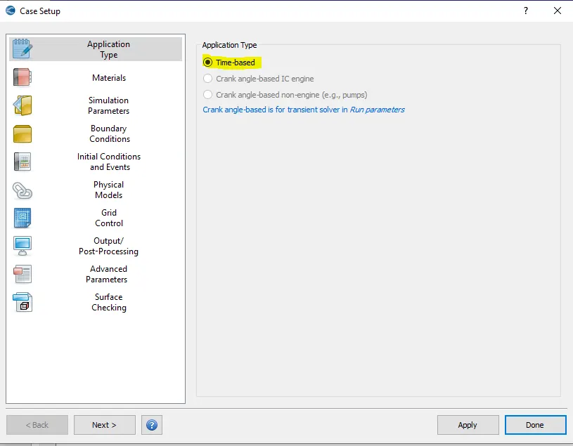
Application Type: Is selected as Time Based

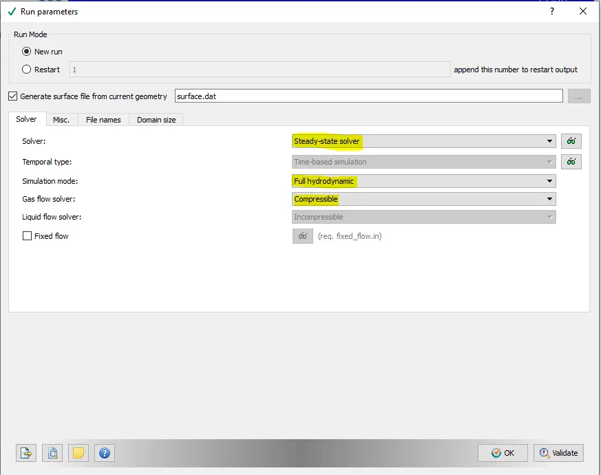
Run Parameters

For the Solver the Steady state solver is selected, simulation mode is full hydrodynamic and Gas flow solver is Compressible.

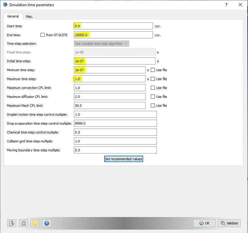
Simulation Time Parameters

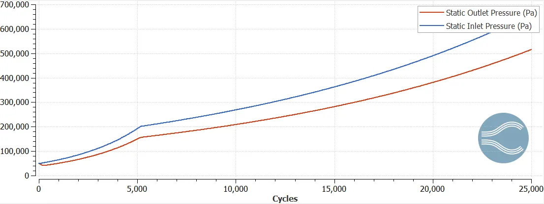
Start time is set to 0, end time is 25000 cycles, Initial and Minimum time step is set to 1e-7 seconds and maximum time step is set to 1 second. Rest all the values are default.

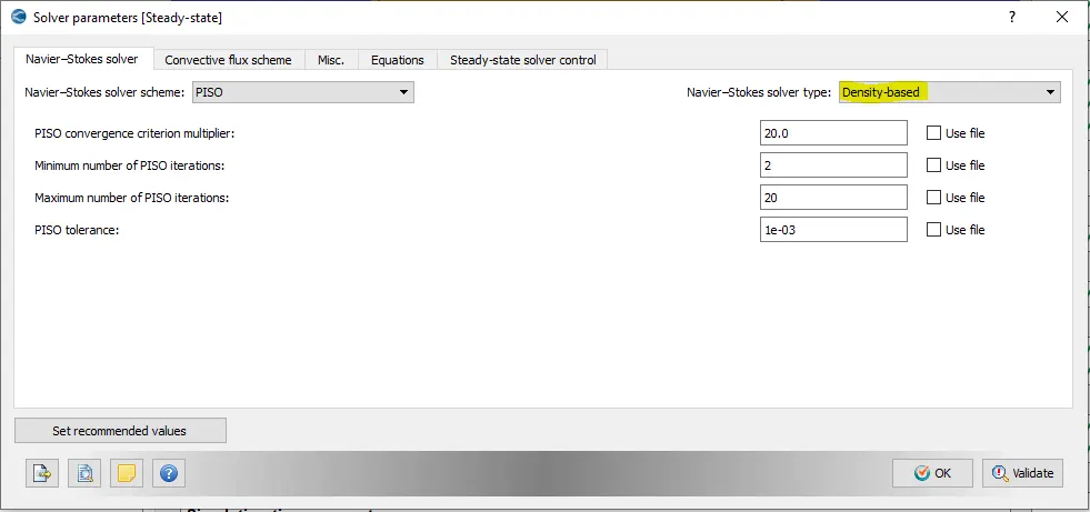
Solver Parameters

All the parameters are default.

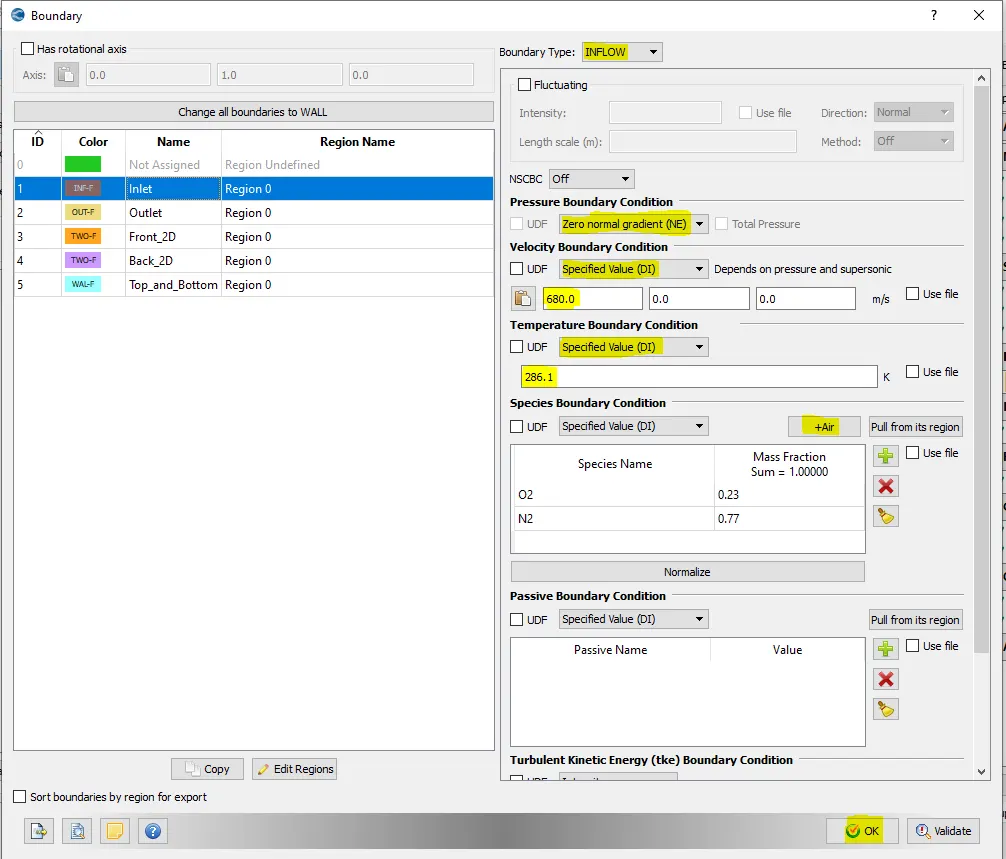
Inlet Boundary

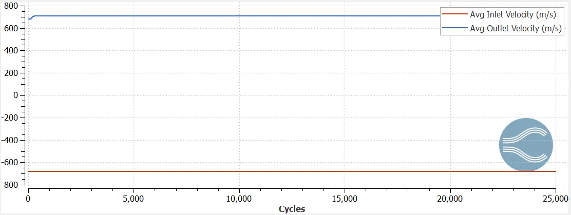
Boundary Type is selected as INFLOW, Pressure Boundary Condition is set to Zero normal gradient (NE), velocity boundary condition is specified value of 680 m/s in X direction.

Temperature boundary condition is set to specified value of 286.1 K. Air is selected for species boundary condition.

Outflow Boundary Condition

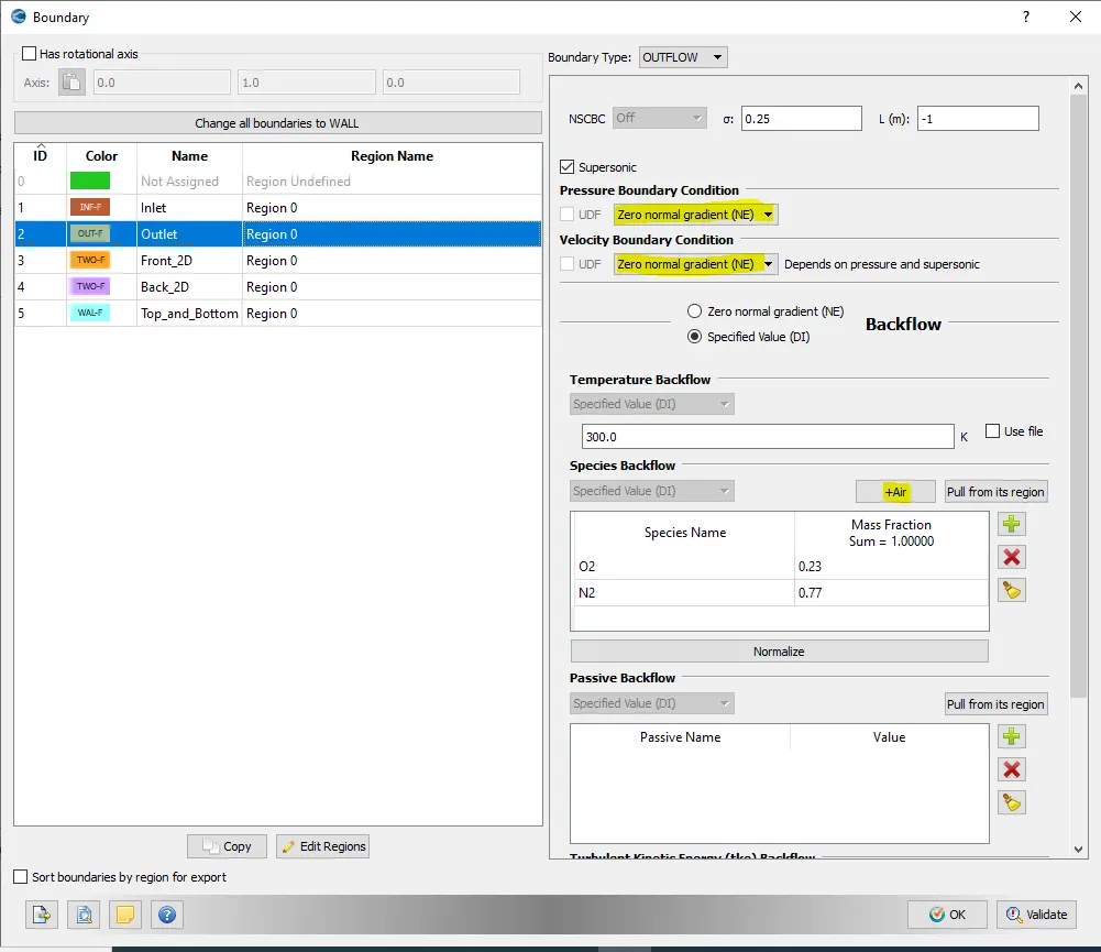
Boundary Type is selected as OUTFLOW, Pressure and velocity boundary conditions are specified as Zero Normal gradient. For Species Backflow Air is selected.

Front and Back Boundary condition

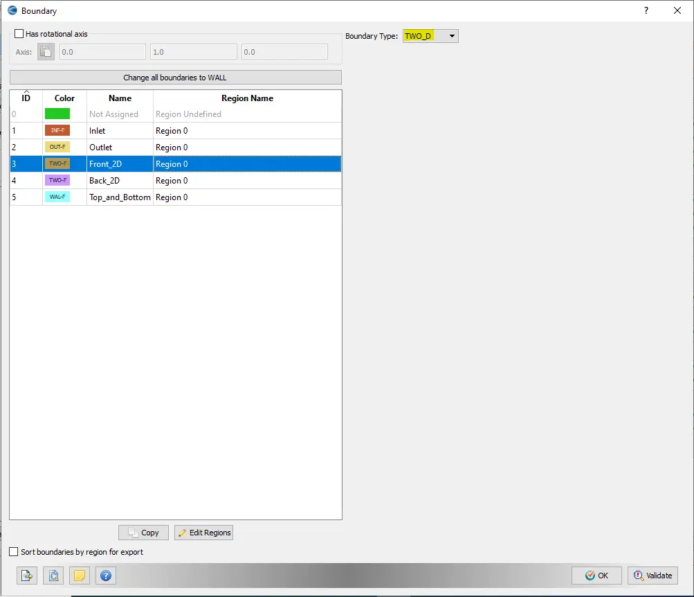
Since this is a 2D problem, the boundary type is specified as TWO_D

Top and Bottom walls

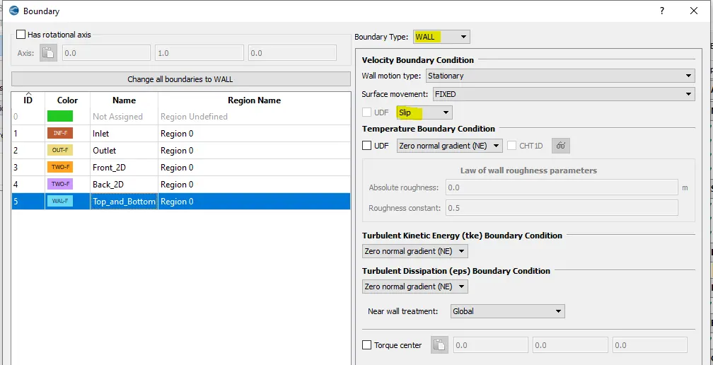
Boundary type is specified as WALL, Velocity boundary condition is Slip type, Temperature boundary condition as Zero normal gradient.

Regions and Initialization

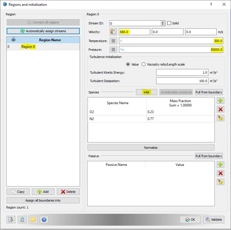
Initial Conditions are velocity = 680 m/s in X direction, Temperature = 300 K, Pressure = 50000 Pa and Species as Air

Turbulence Modeling

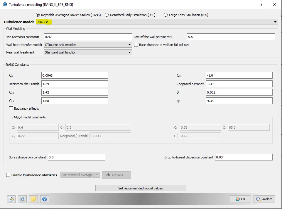
Turbulence model is RNG k-epsilon and all parameters are kept default.

Grid Control

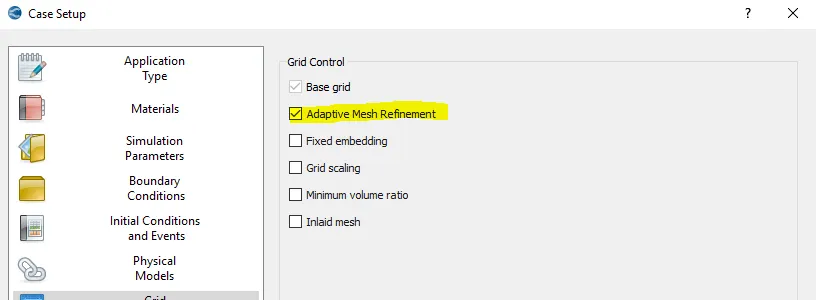
Adaptive Mesh Refinement enabled in Grid Control

Base Grid Size

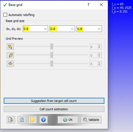
Base Grid size is set to 0.8 m for a bounding box dimensions of 65 x 45.15 x 8.15 m

Adaptive Mesh Refinement

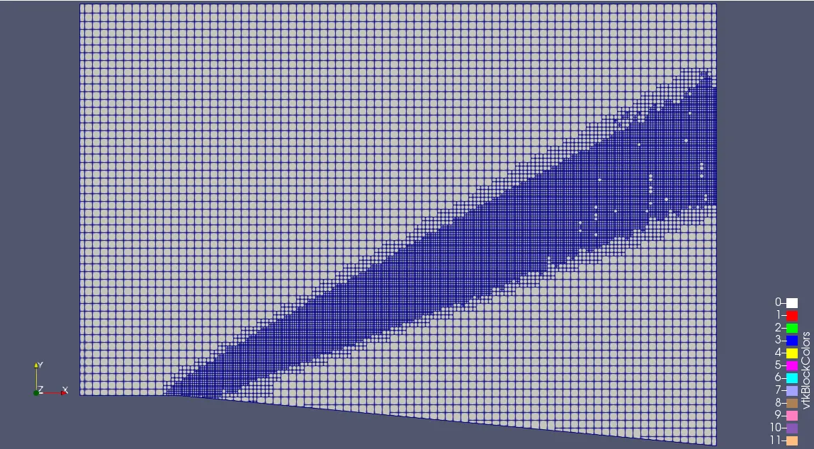
Minimum cells set to 1 and Maximum cells set to 200000, Temperature scheme is used for AMR with Embed type as SGS (Sub Grid Scale), max embedding level as 2, Sub grid criterion is varied for every case.

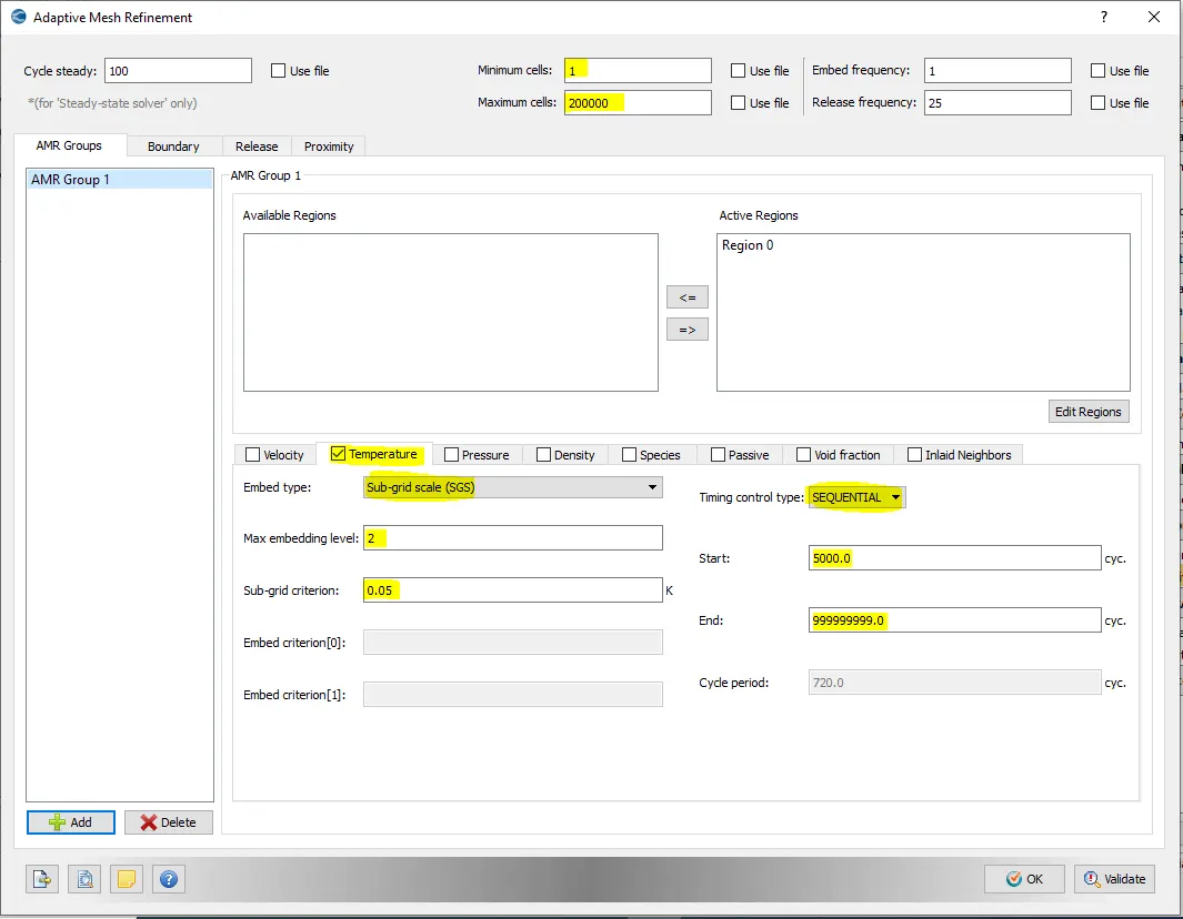
The adaptive mesh refinement option refines the mesh in those areas where the second order derivative of temperature `{del^2T}/{delx^2}` is fluctuates more than the SGS parameter value. This option captures the flow physics more accurately by refining the mesh locally in those areas where there are abrupt changes in the feild variables (pressure, temperature, velocity, density). In this case we have choosen the temperature variable to refine the mesh locally.

Output Files

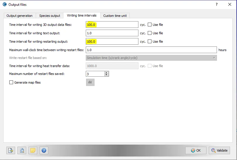
Time interval for writing 3D output files and restarting output changed to 100.

Four cases were setup

Case 1: Velocity = 680 m/s (Supersonic flow) and SGS parameter = 0.05

Case 2: Velocity = 680 m/s (Supersonic flow) and SGS parameter = 0.01

Case 3: Velocity = 680 m/s (Supersonic flow) and SGS parameter = 0.1

Case 4: Velocity = 100 m/s (Subsonic flow) and SGS parameter = 0.05

Results of Simulation

Case 1: Velocity = 680 m/s and SGS = 0.05

Mesh

Pressure Contour Plot

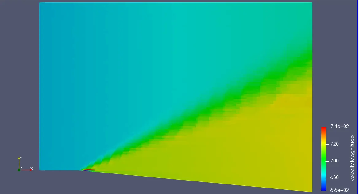
Velocity Contour Plot

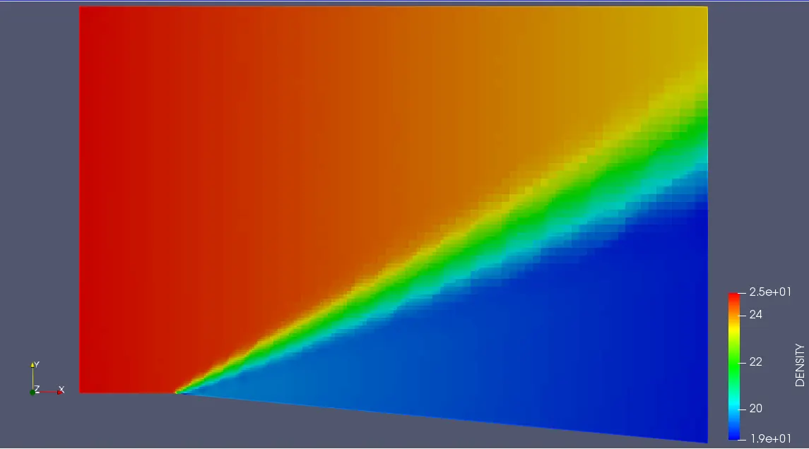
Density Contour Plot

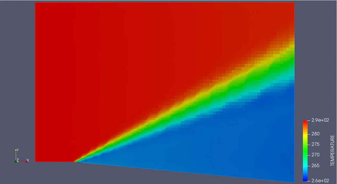
Temperature Contour Plot

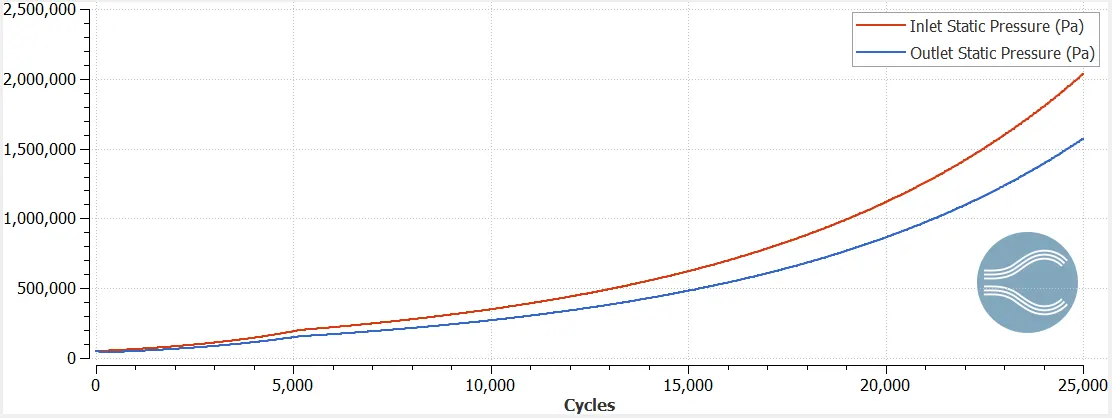
Static Pressure

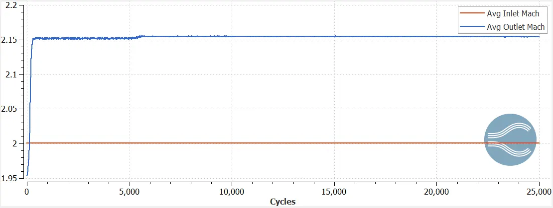
Mach Number

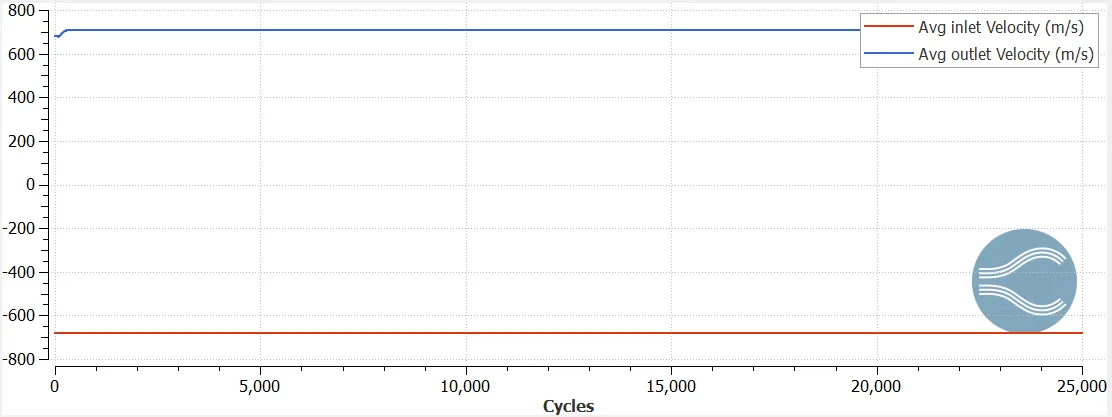
Velocity

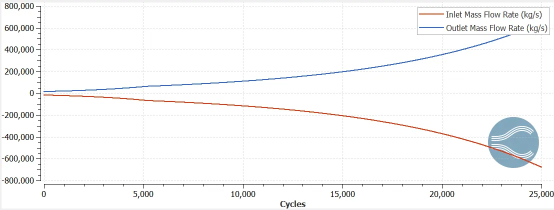
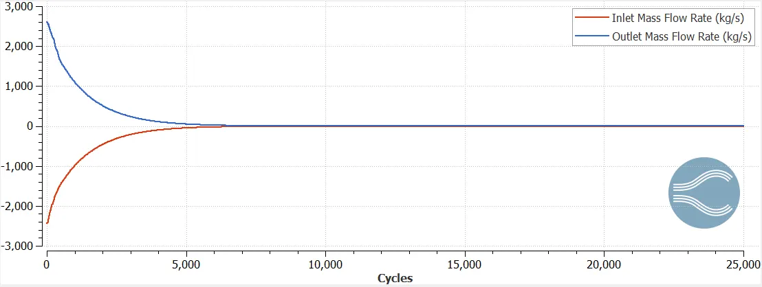
Mass Flow Rate

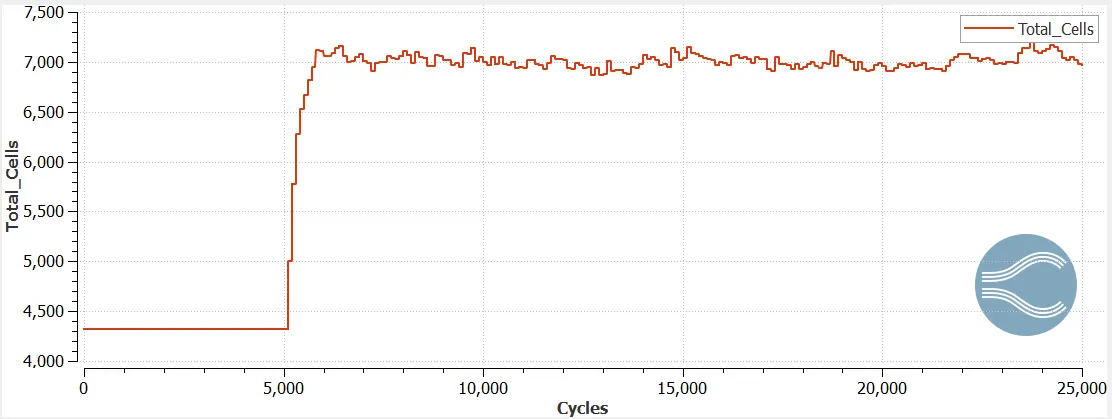
Total Cell Count

Case 2: Velocity = 680 m/s and SGS = 0.01

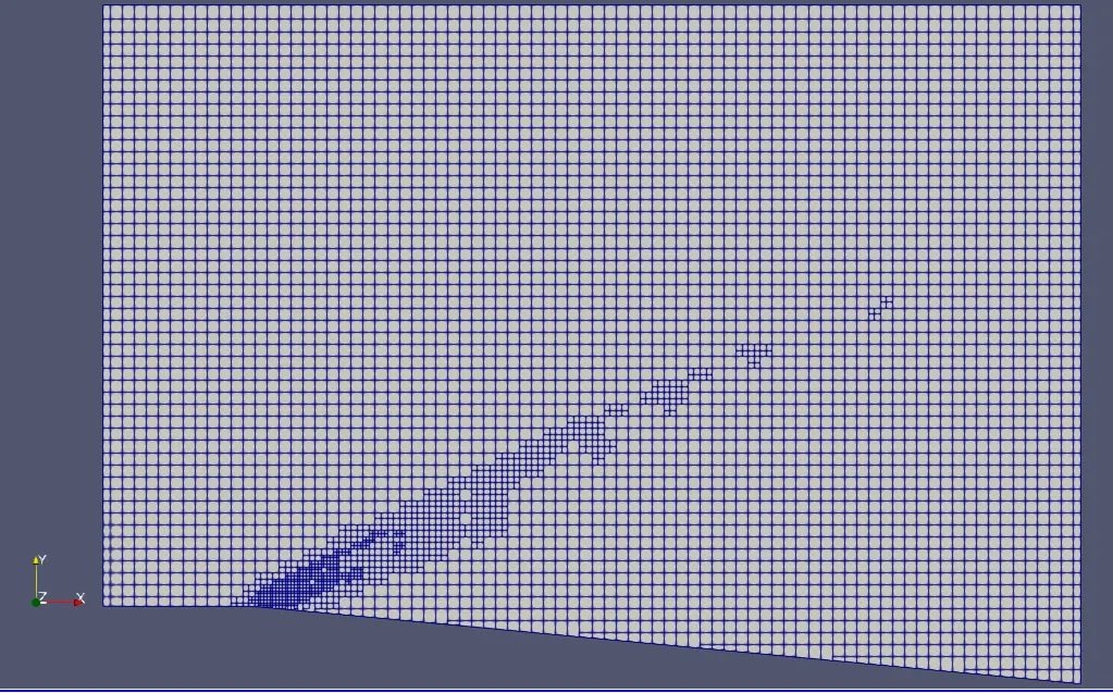
Mesh

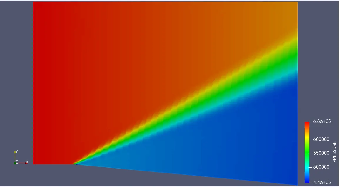
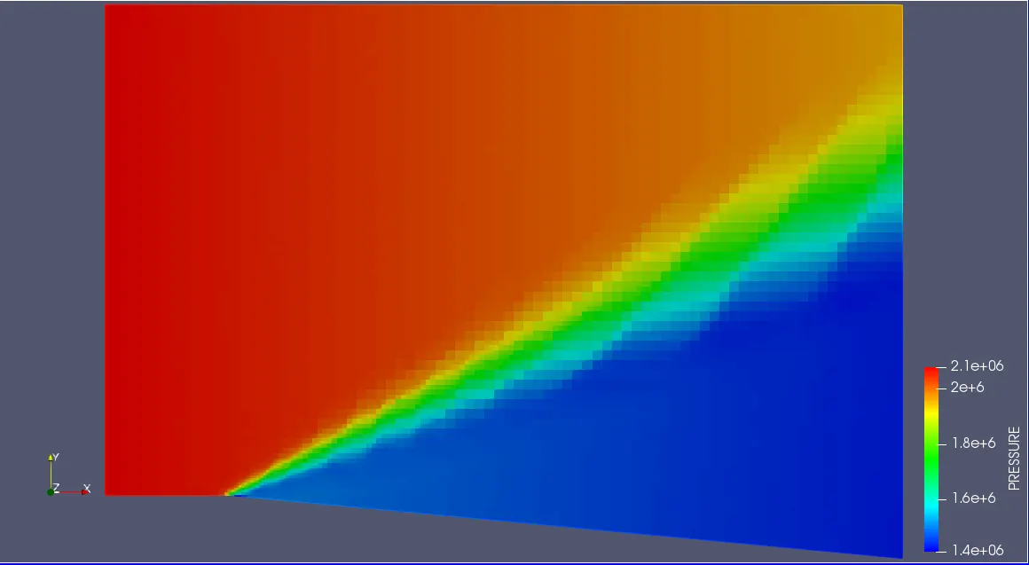
Pressure Contour

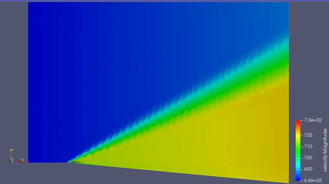
Velocity Contour

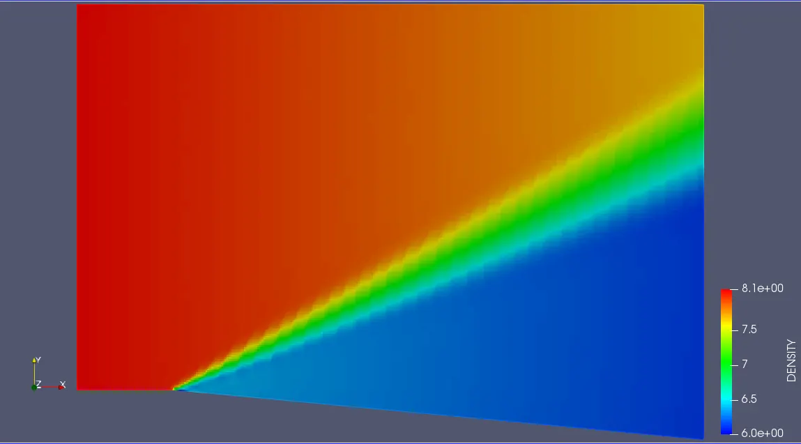
Density Contour

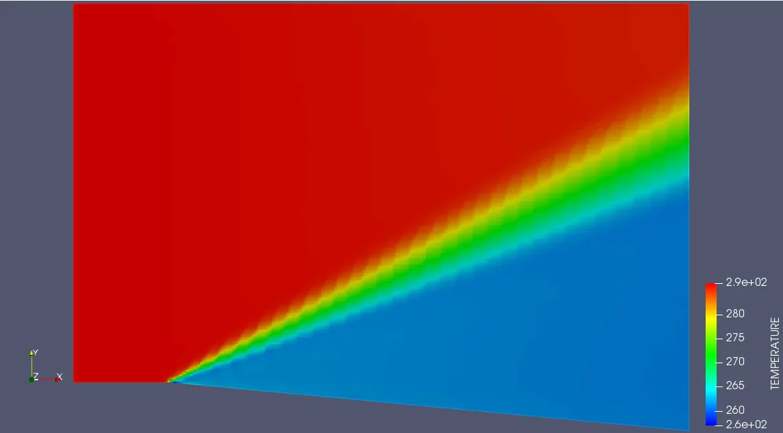
Temperature Contour

Static Pressure

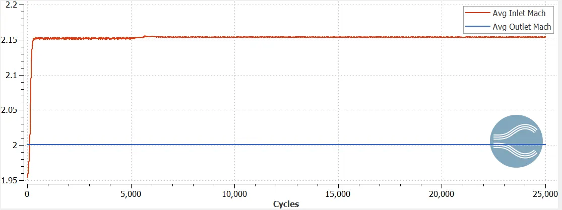
Mach Number

Velocity

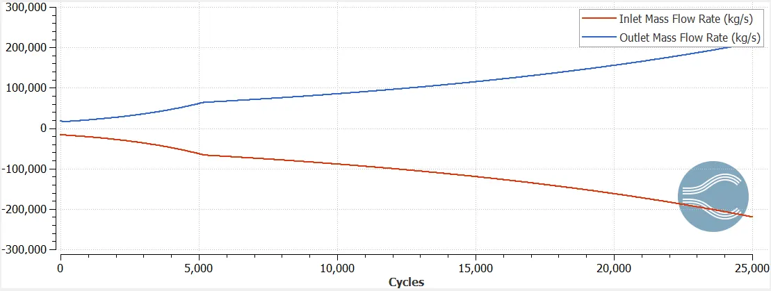
Mass Flow Rate

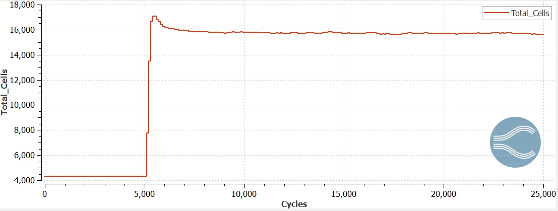
Total Cell Count

Case 3: Velocity = 680 m/s and SGS = 0.1

Mesh

Pressure Contour

Velocity Contour

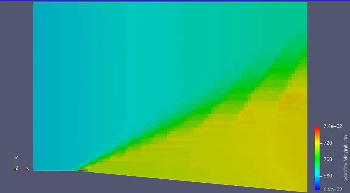
Temperature Contour

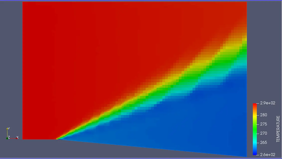
Density Contour

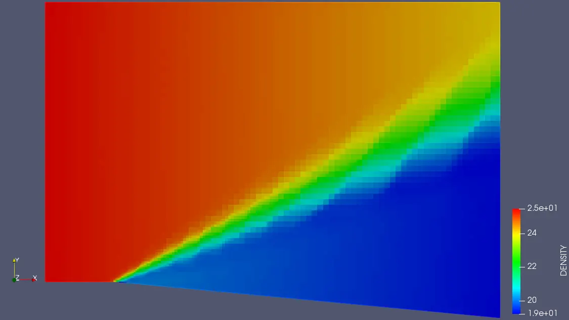
Static Pressure

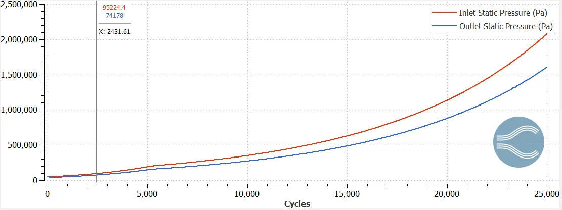
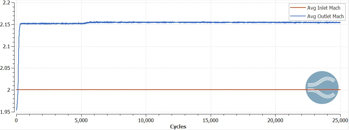
Mach Number

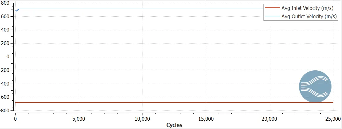
Velocity

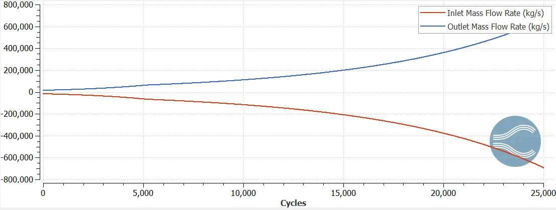
Mass Flow Rate

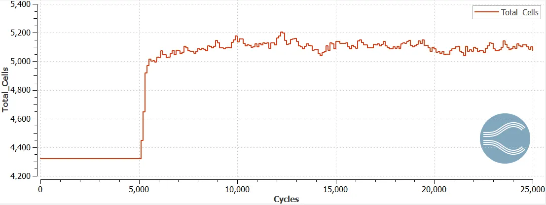
Total Cell count

Case 4: Velocity = 100 m/s and SGS = 0.05

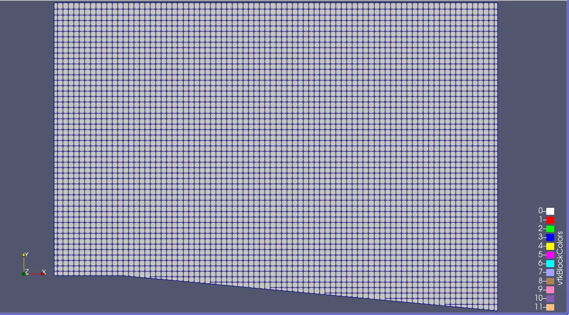
Mesh

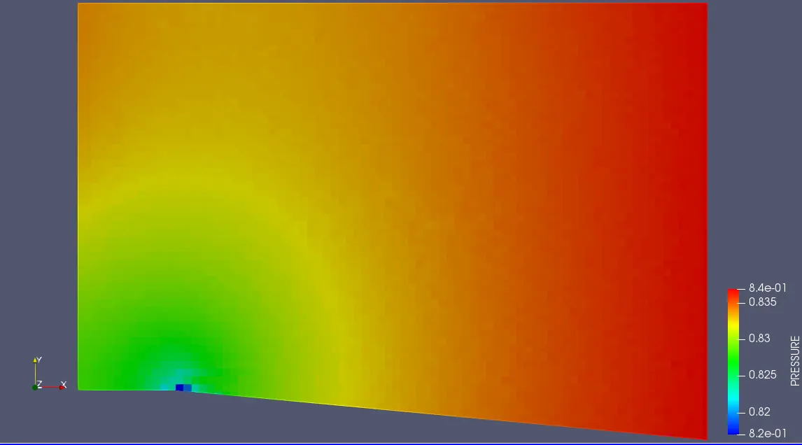
Pressure Contour

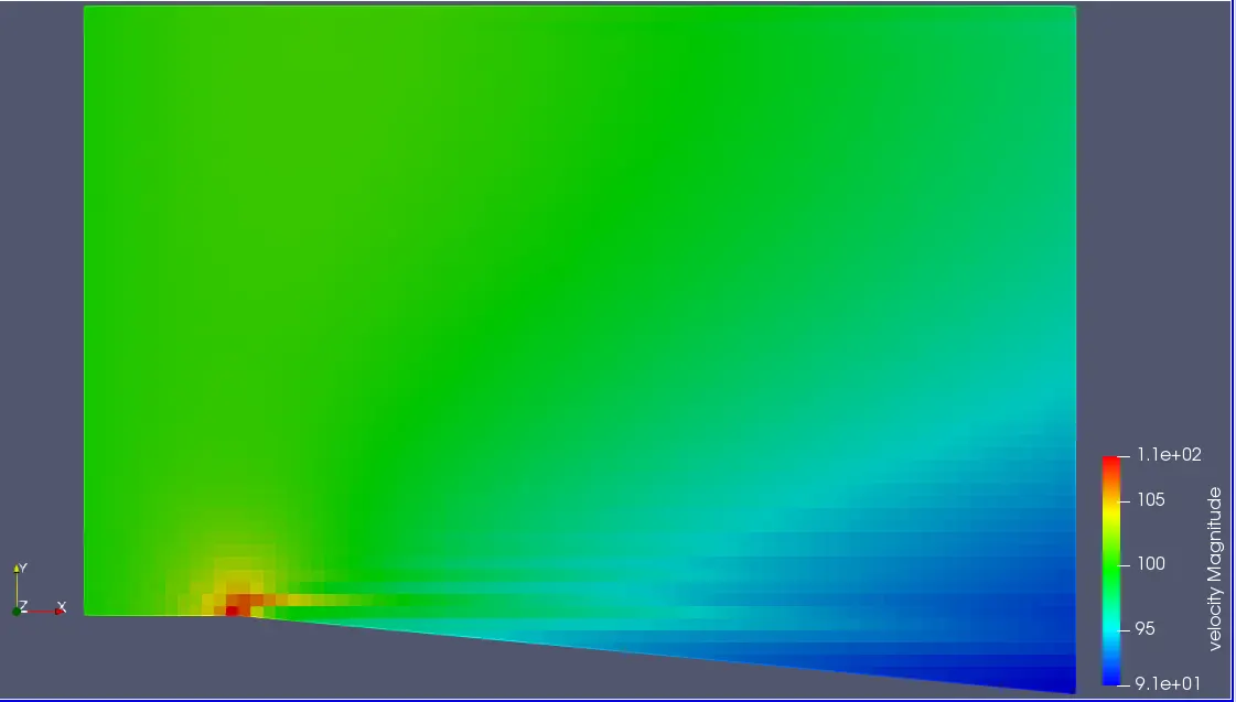
Velocity Contour

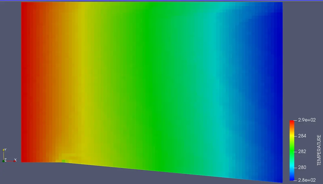
Temperature Contour

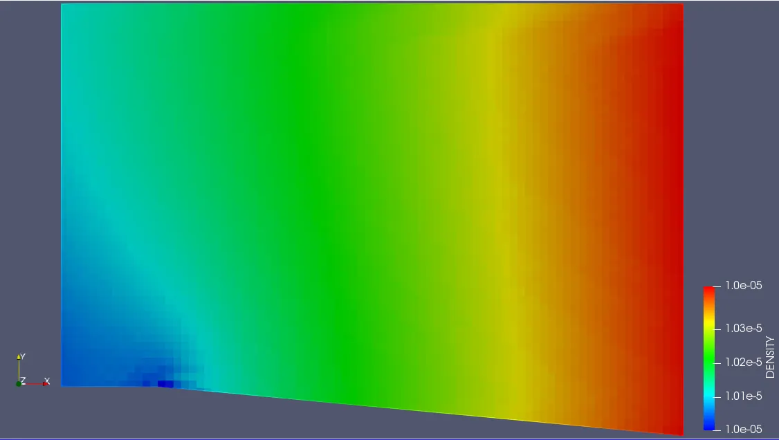
Density Contour

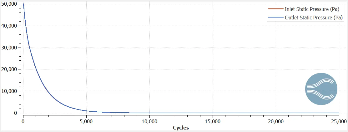
Static Pressure

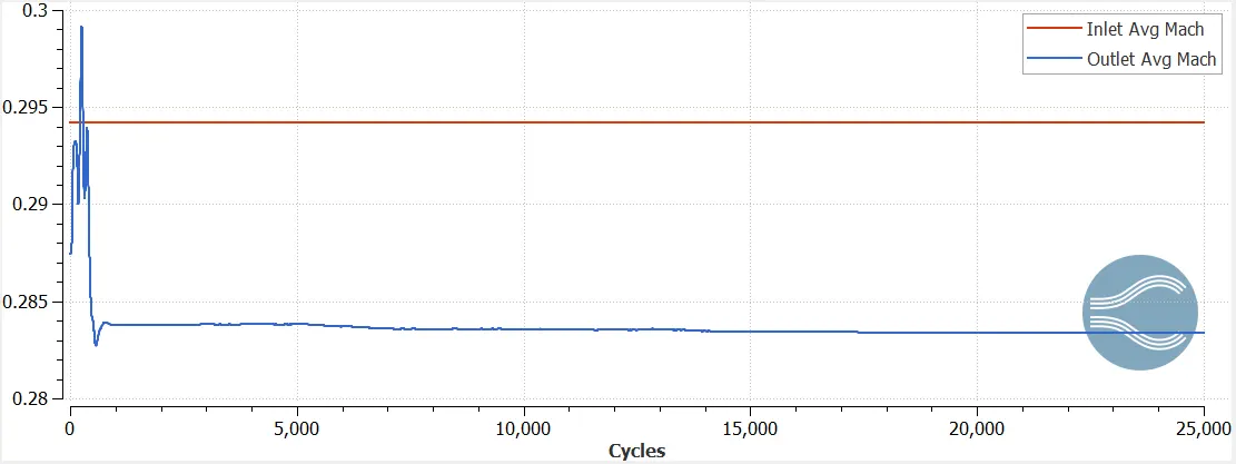
Mach Number

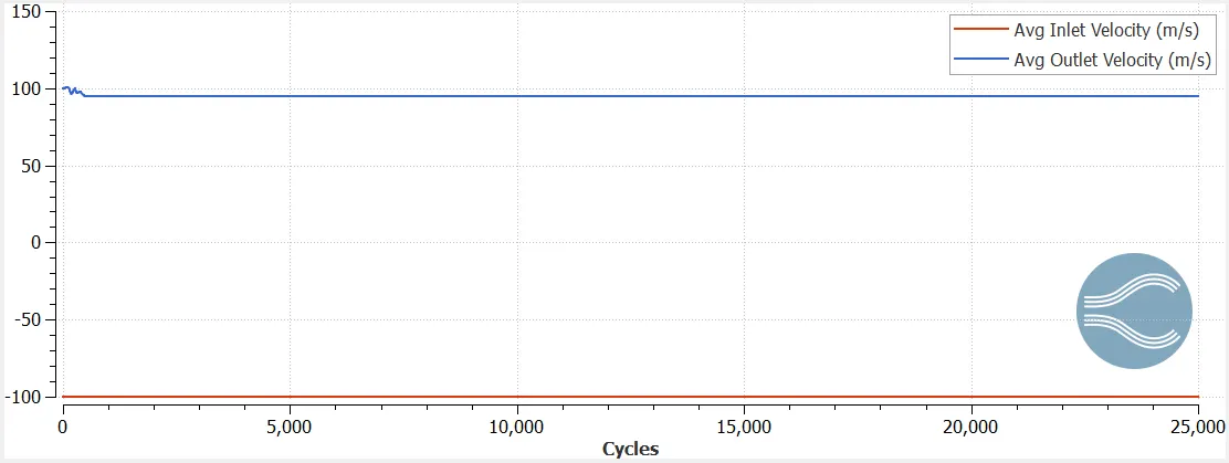
Velocity

Mass Flow Rate

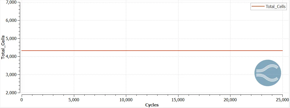
Total Cell count

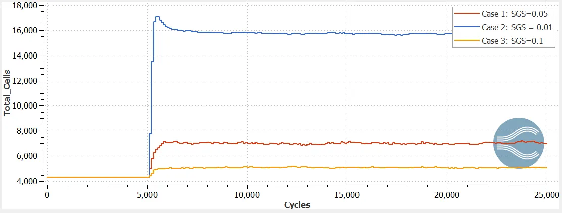
Effect of SGS Parameter on Total Cell Count

Observation from the above plots

Effect of SGS parameter on shock location and Total cell count

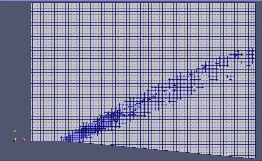
1. Cell count: As the SGS parameter decreases, the total cell count increases. In other words, for small SGS parameter, AMR refines the mesh for more number of cells in and around the shock waves.

2. Shock Location: For a high SGS parameter, the mesh refinement area (as seen on the mach fan) is very small like in Case 3 (SHS = 0.1) and for the a small SGS parameter, the mesh refinement area spans from the sharp edge till the outlet boundary.

Subsonic Vs Supersonic Flow Comparison

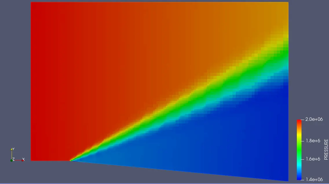
In supersonic flow, the prandtl-meyer expansion fan is clearly visible and the mesh refinement is also visible in the shock region

Whereas on the other hand, in case of a subsonic flow, the prandtl-meyer expansion fan is not at all visible and even the mesh refinement is not visible. This is because there are no sudden fluctuations in pressure, velocity, temperature or density or in other words shock.

Also the average Mach number increases from the inlet to the outlet in case of supersonic flow and decreases in case of subsonic flow.

Conclusions

i. The AMR feature is better able to capture the expansion fan as compared to the base grid.

ii. Although the tip of the expansion fan is located near the sharp corner for all cases, its resolution increases with a decrease in the SGS criterion. For greater values of SGS criterion, the tip becomes diffused.

iii. The gradients - across the expansion fan - are better captured by simulations having small values of SGS criterion.

iv. With an increase in SGS criterion, the total cell count decreases.