TRANSIENT SIMULATION OF AIR FLOWING OVER A ROTATING THROTTLE BODY IN AN ELBOW USING CONVERGE CFD

Introduction:

The throttle body assembly is a well-known part of the IC engine. The main function of the throttle body assembly is to control the airflow into the engine cylinder based on vehicle demand. It is also known as a butterfly valve. Amount of fluid goes through the butterfly valve is decided by the angle of the disc.

These Valves are used in a wide range of applications. The typical applications of Butterfly valves are,

• Carburettors
• Fire fighting devices and Apparatus
• Thermal power stations

The angle of the throttle valve plays the main role in control the mass flow rate of the fluid. As we know, an increase in angle leads to the increase in mass flow rate. The similar results are achieved through this transient analysis.

In this analysis, two-position of throttle valve were used with different time duration. For 0 to 2 ms, the angle of the throttle is going to rotate from 0 degree to 25 degree and then the angle of the throttle remains unchanged till 4 ms. Then the throttle will come back to the original position at 6 ms.

Objective:

To perform the Transient simulation of flow over a throttle body using Convergent Science Software to find out the variation of mass flow rate at different valve positions.

Introduction to Throttle valve :

Butterfly Valve

Throttle

A throttle is a mechanism through which fluid flow is controlled by obstructing the flow. In an IC engine, the throttle controls the engine power in response to driver accelerator pedal input by regulating the amount of air entering the engine cylinder. It is a butterfly valve to control the air flow.

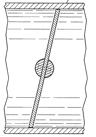
While designing a fuel management system for an SI engine, the amount of air flowing in the cylinders is very important. Performance and emission reduction can be improved by designing and testing a fuel management system in a computer environment and it can also save valuable setup time in an engine test cell. One important part of the modeling is the throttle which regulates the air. In this project, steady state air flow over a throttle body is simulated in Converge CFD.

Mesh details:

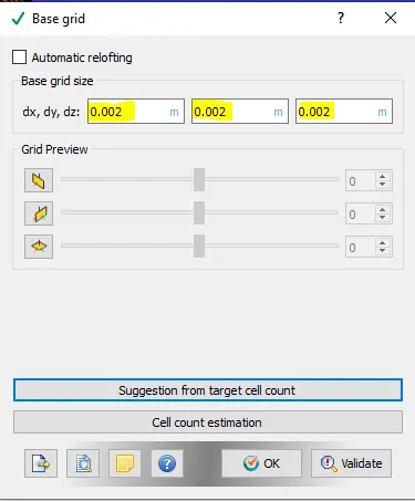
• Element size, dx = dy = dz = 2 mm
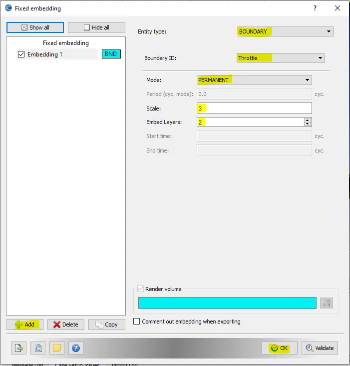
• The fixed embedding is created to capture more cells near the throttle body.
• Number of layers = 2
• Scale = 3
• Converge uses Adaptive mesh refinement to maintain a given mesh property at different valve positions.

Case Setup:

Case Setup:

1. First thing to be done is geometry cleanup. The flow is to be simulated inside the elbow so the thickness of the elbow must be converted to the flow region.

For that to be done, delete the outer face and the two thickness faces of the elbow. Use the "By Angle" option shown below to select the faces and then press D to delete the faces.

To use the HotKeys, the Key icon must be enabled.

2. Create patches for inlet and outlet faces.

In the geometry editing toolbox, go to Repair > Patch > Free Edge Loop > By Open Edge > Select the edges and press apply.

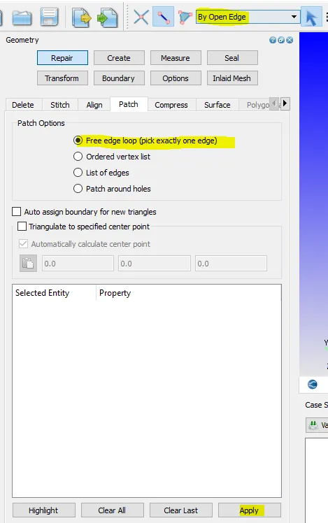
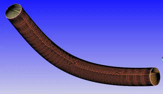
The patches should be formed on both the ends of the elbow as shown below.

3. Create and assign boundary flags

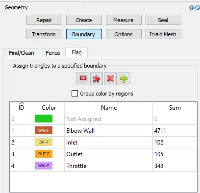
Go to Boundary > Flag > Plus icon and create 4 boundary flags and assign the flags to their respective geometry.

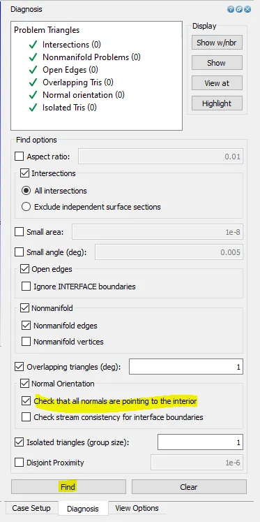
4. Run a diagnosis check to ensure that there are no errors. Enable "Check that all the normals are pointing to the interior"

5. Case Setup:

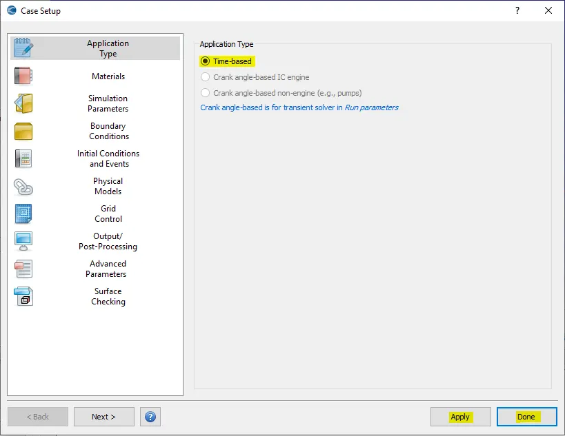
5.1 Application Type

Select Time Based

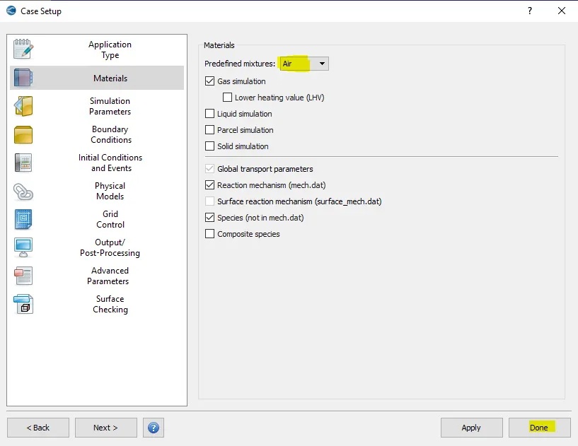
5.2 Materials

For predefined mixtures select Air and keep Gas Simulation enabled.

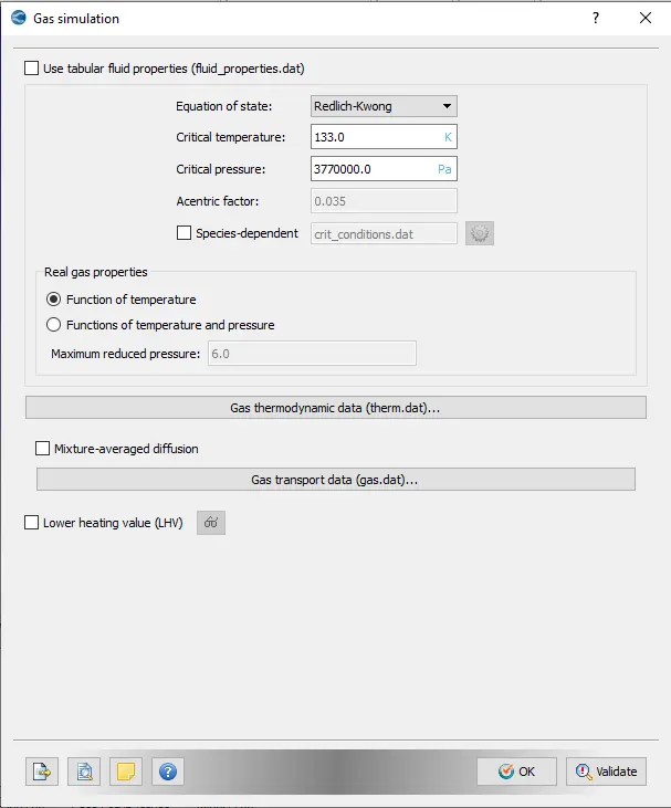
5.3 Gas Simulation

Keep the default values and Press OK

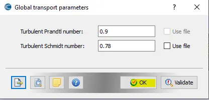
5.4 Global Transport Properties

Keep all the values default and press OK

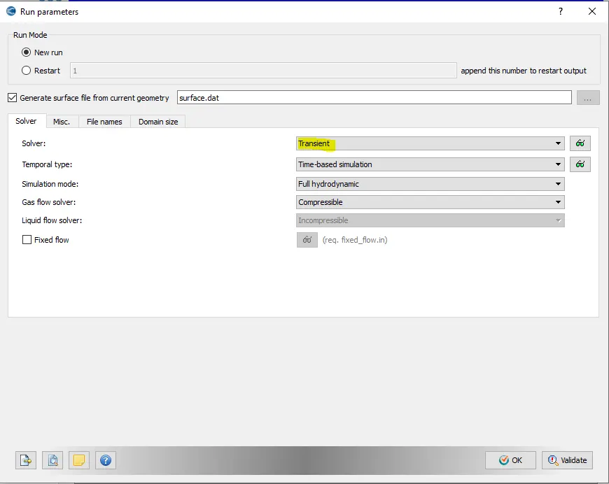
5.5 Run Parameters

Select the solver as Transient

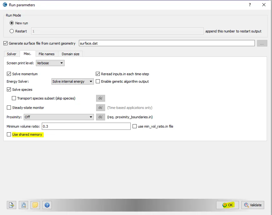
under Misc. tab disable use shared memory and press OK.

5.6 Simulation Time Parameters

End Time Calculation

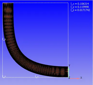
The encumbrance dimensions in x and y directions are roughly 0.1 metres. Length of pipe will not be more than 0.1*2 = 0.2 metres.

The average velocity at inlet was 225 m/s in the steady state simulation.

So, Flow through time = Characteristic Length / Average Velocity = 0.2 / 225 = 8.8888e-4 seconds or 0.8888 milliseconds

We choose to simulate the flow till roughly 10 times the flow through time 0.888*10 = 8.88 milliseconds

We round off the end time to 10 milliseconds.

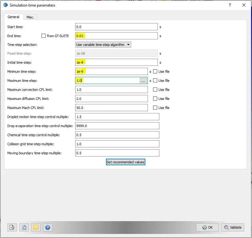
Select start time as 0 seconds, end time as 0.01 seconds, Initial and Minimum time step as 1e-9 seconds and Maximum time-step as 1 second. Keep all the other values default and Press OK.

5.7 Solver Parameters

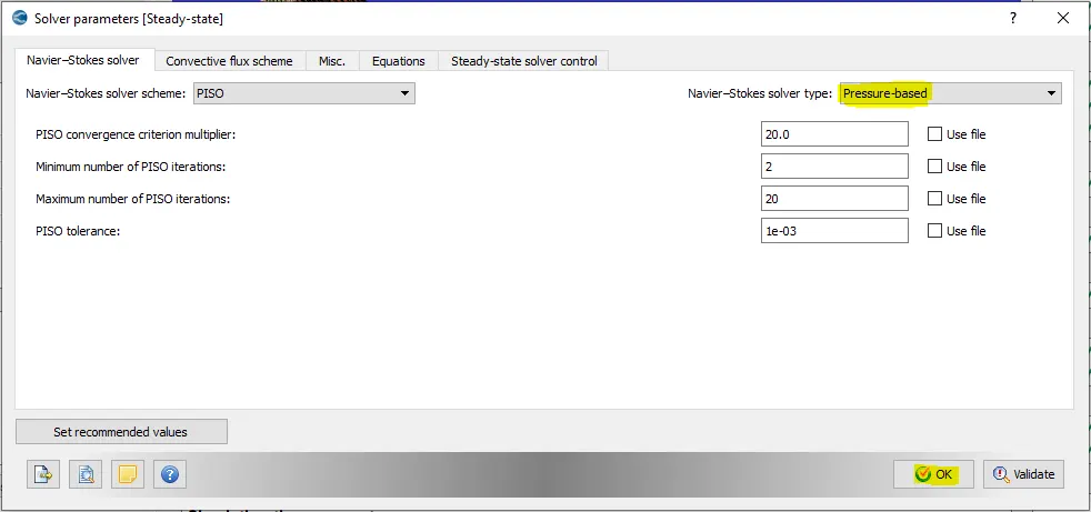
Change the Navier-stokes solver type as Pressure-based, keep all other settings as default and press OK.

5.8 Regions and Initializations

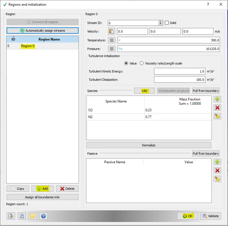
Select Add to create a new region. Select Air for Species initial conditions and keep the other values default and Press OK.

5.9 Turbulence Modeling

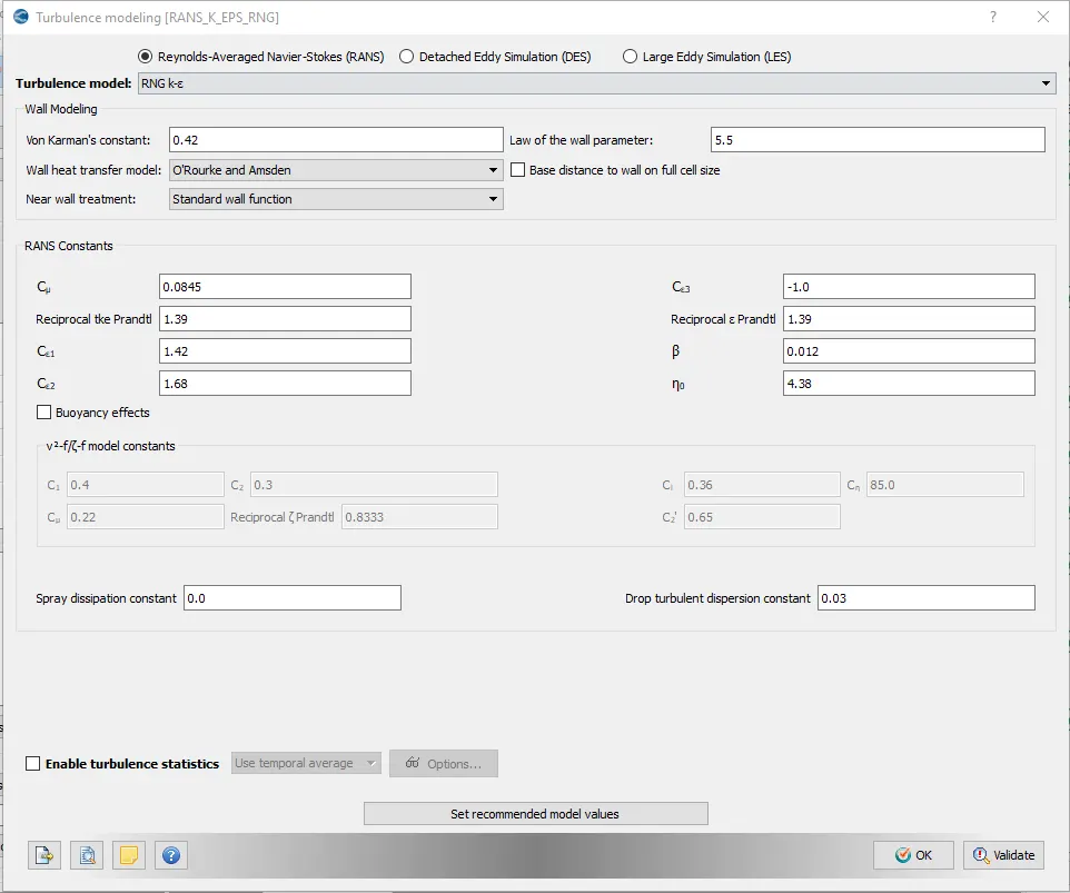
Keep all the settings default and press OK.

5.10 Grid Control

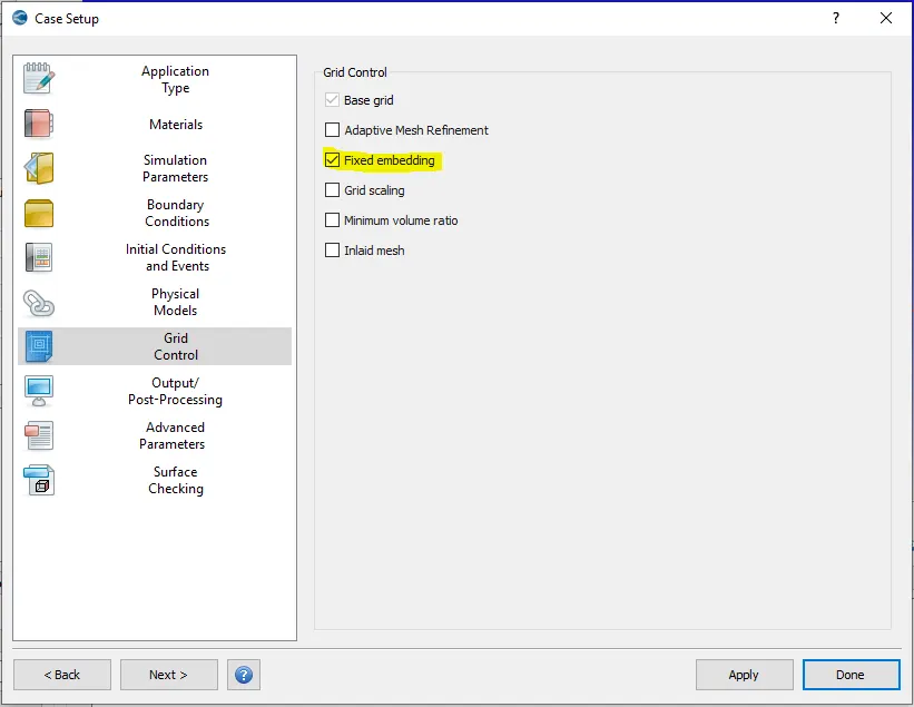
Enable Fixed Embedding.

5.11 Base Grid

Keep the mesh size as 2mm.

5.12 Fixed Embedding

Select Add, set Entity type as BOUNDARY, set Boundary ID as Throttle, scale as 3 and Embed Layers as 2.

5.13 Boundary

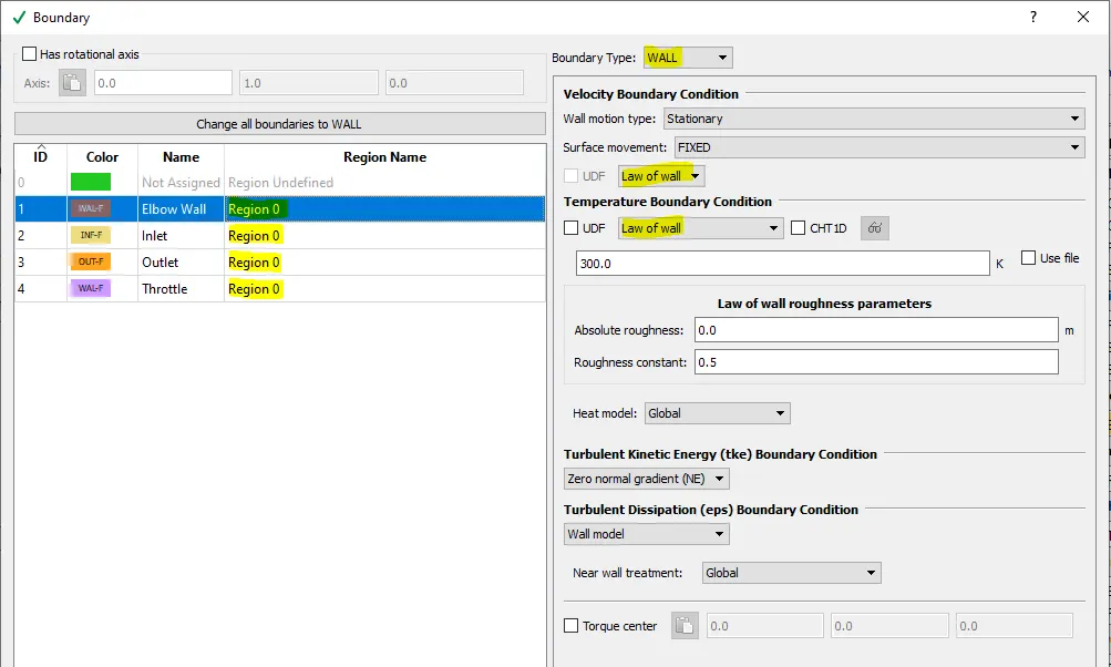
For Elbow Wall, select the boundary type as WALL, keep Law of wall for both Velocity and Temperature boundary condition and keep the other settings default as shown below.

Keep the Region Name as Region 0 for all the boundaries.

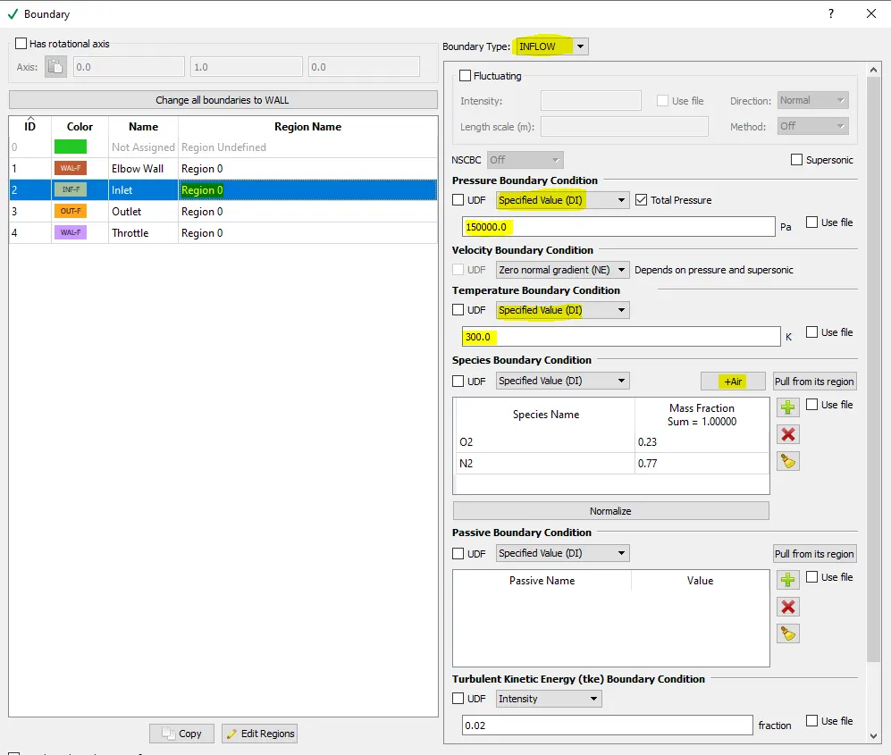
For Inlet boundary select the Boundary Type as INFLOW, specify the Pressure boundary condition as specified value of 1.5e5, keep the temperature boundary condition as default, and for species boundary condition select air

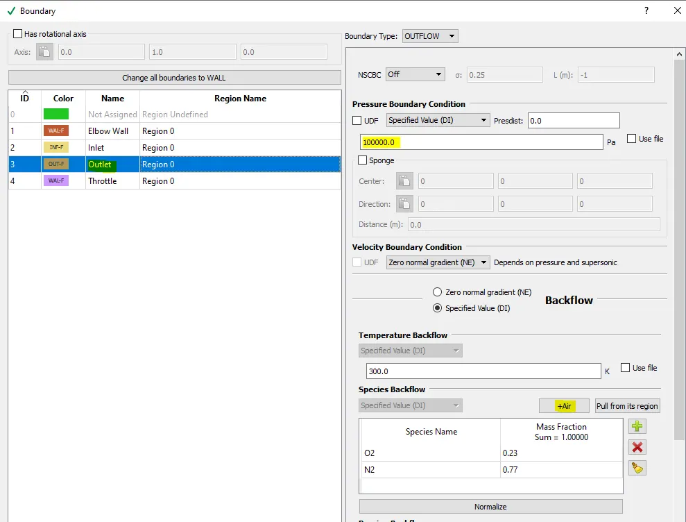
For Outlet set the Pressure Boundary condition as Specified Value of 1e5 and for species backflow select Air, keep the other settings default.

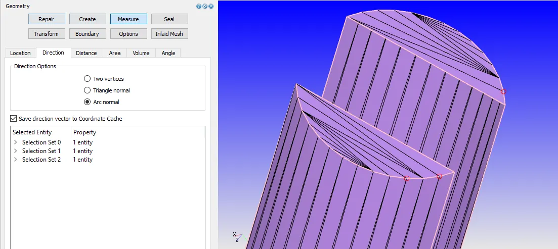
Measure the Rotation axis and centre for throttle

GO to Measure > Direction > Arc Normal > Select three points on the arc and press apply.

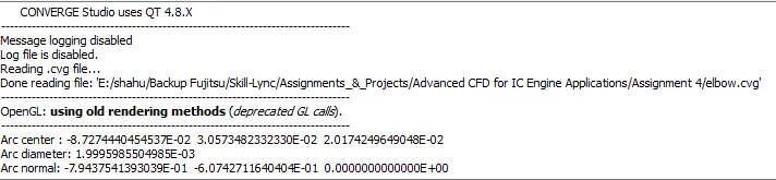
After pressing apply, the measured values will get printed in the Message Log of Converge Studio as shown below.

For Throttle boundary select the boundary type as WALL, the Wall motion type as Rotating and keep the velocity and temperature boundary condition as law of wall.

For Rotation Centre use the Arc Centre values measured in the previous step and for the Rotation axis use the Arc Normal values measured in the previous step.

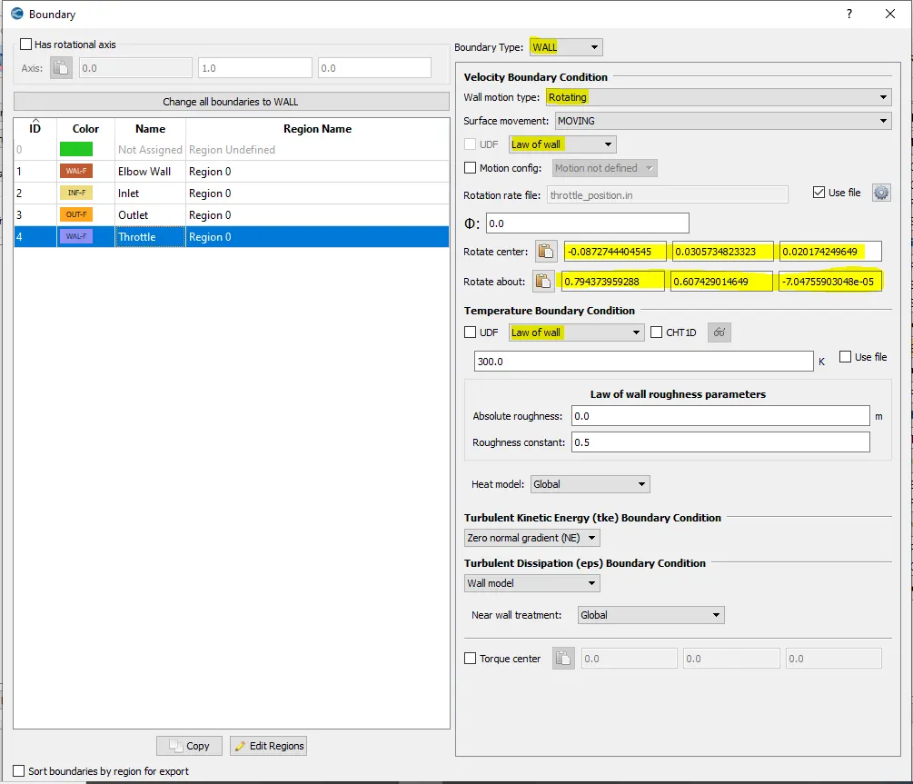
For Rotation Rate, click on Use File. Then enter the values shown in the below image.

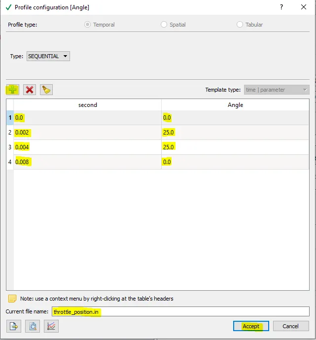
We want the throttle to rotate from 0 to 2 ms by 25 degrees, then remain stationary till 4 ms and finally rotate to its original position by 8 ms.

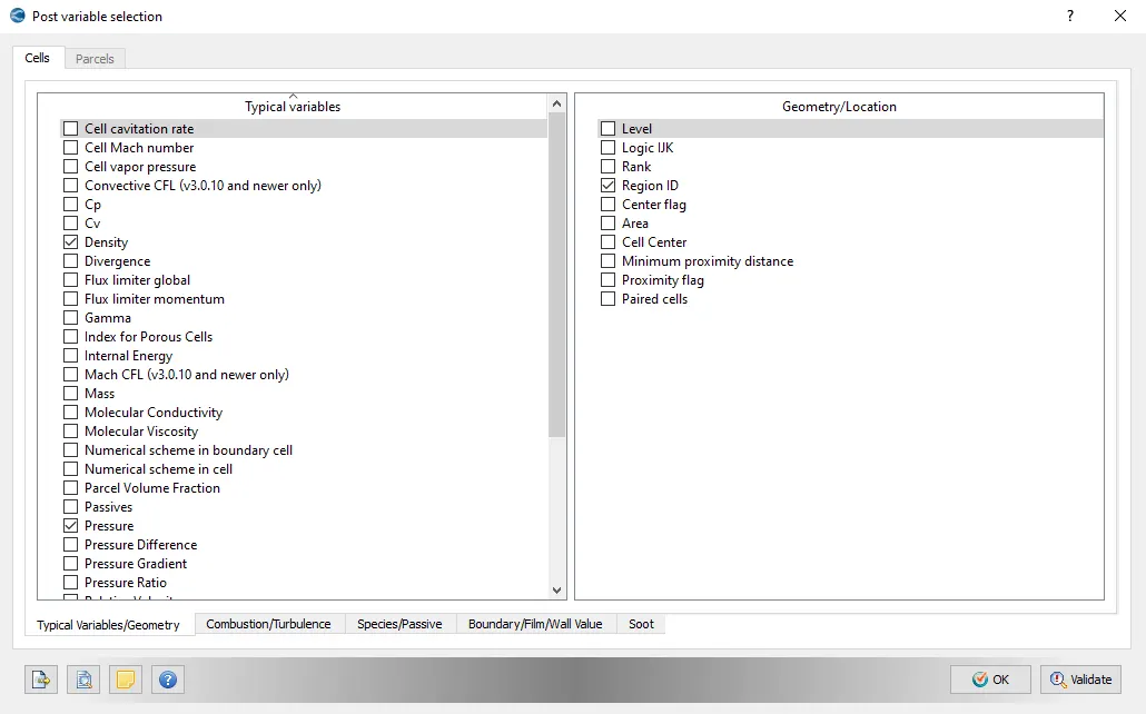
5.14 Post Variable Selection

Keep all the settings default and press OK.

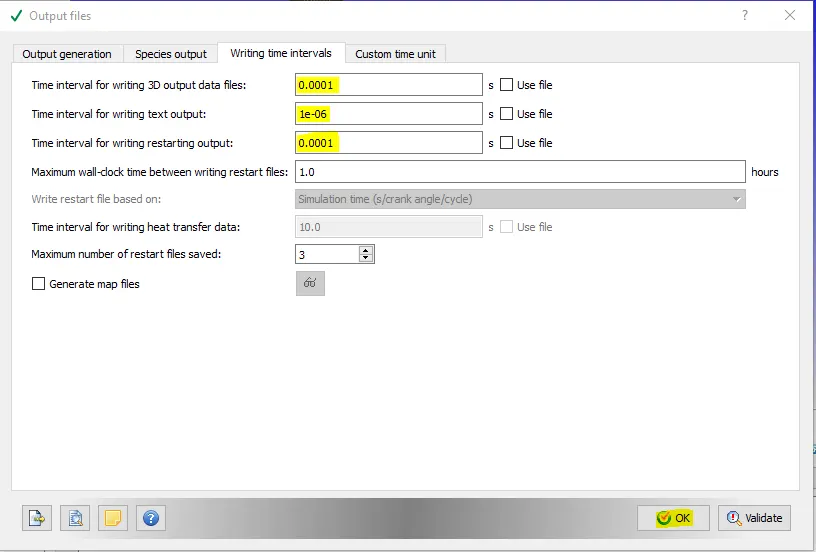
5.15 Output Files

Change the time interval for writing 3D output data files and interval for writing restarting output to 0.0001 and keep all the other values default and press OK.

Total time is 10 milliseconds and we want atleast 100 3D output data files to produce a smooth animation.

So, time interval for writing 3D output data files = 0.01/100 = 0.001 seconds

6. Export all the input files

Export all the input files into a separate folder

Top Panel Files > Export > Export Input Files

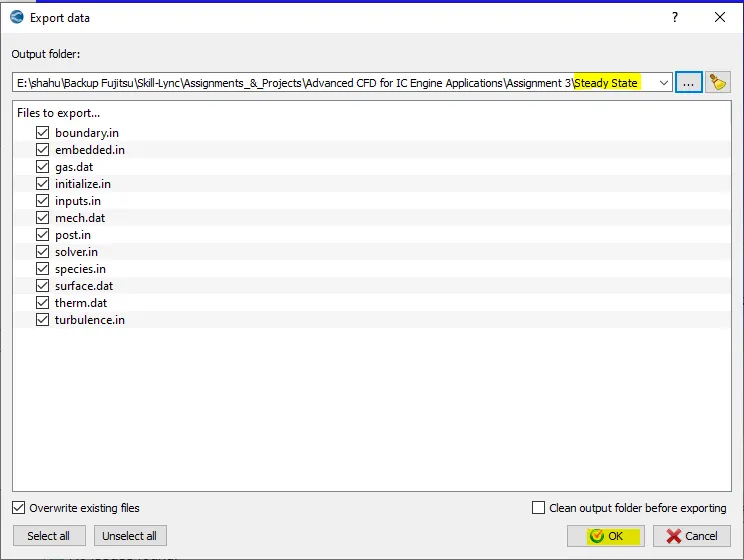
Set the export directory and press OK.

7. Run the simulation

Copy the mpiexec.exe file to the directory in which the input file was exported in the previous step.

Open Cygwin and navigate to that directory and enter the below command to start the simulation.

mpiexec.exe -n 3 "C:Program FilesConvergent_ScienceCONVERGE3.0.12binconverge-intelmpi.exe" restricted </dev/null> logfile.txt &

8. Post Convert the Output Files to Paraview VTK inline binary format

After the simulation run is complete navigate to the output folder and enter the below command in cygwin.

mpiexec.exe -n 4 post_convert_30_msmpi_64.exe

After that enter the Case Name press Enter

Then type 8 and press enter to select the paraview format.

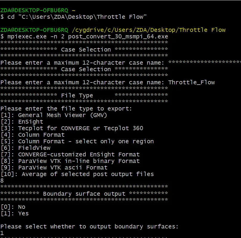
For boundary surface output type 1 and press enter

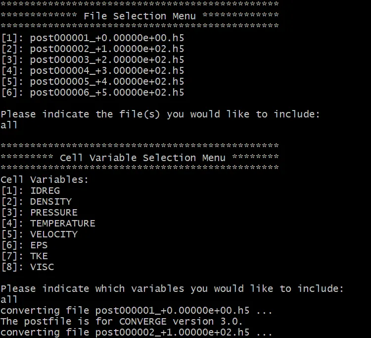
Type all and press enter to post convert all the files. Repeat the same for the Cell variable selection menu. All the files will be converted to paraview format.

9. Launch Paraview and open the .vtm file.

No hydrodynamic simulation to check mesh :

Results of Simulation

Mesh

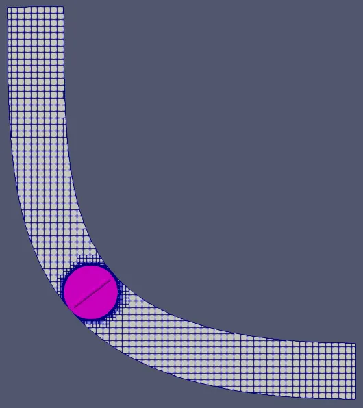
A closer look at the mesh near the throttle region.

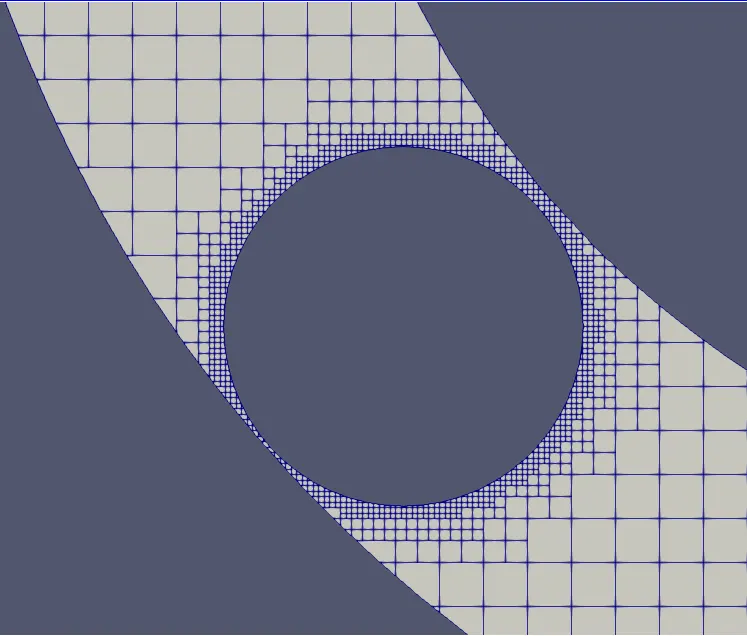
Observe how the mesh is refined near the throttle boundary and how the mesh size gradually increases as we move away from the throttle. This is the benefit of using Fixed Embedding in Converge.

Pressure and Velocity Contours

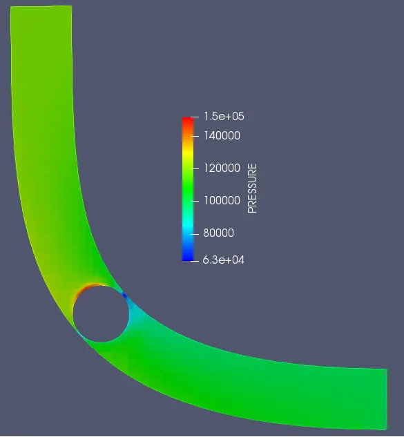
Pressure Contour (at throttle angle = 0 degrees)

The below image shows a pressure contour plot on a slice of the elbow pipe.

A closer look at the pressure contour plot near the throttle region

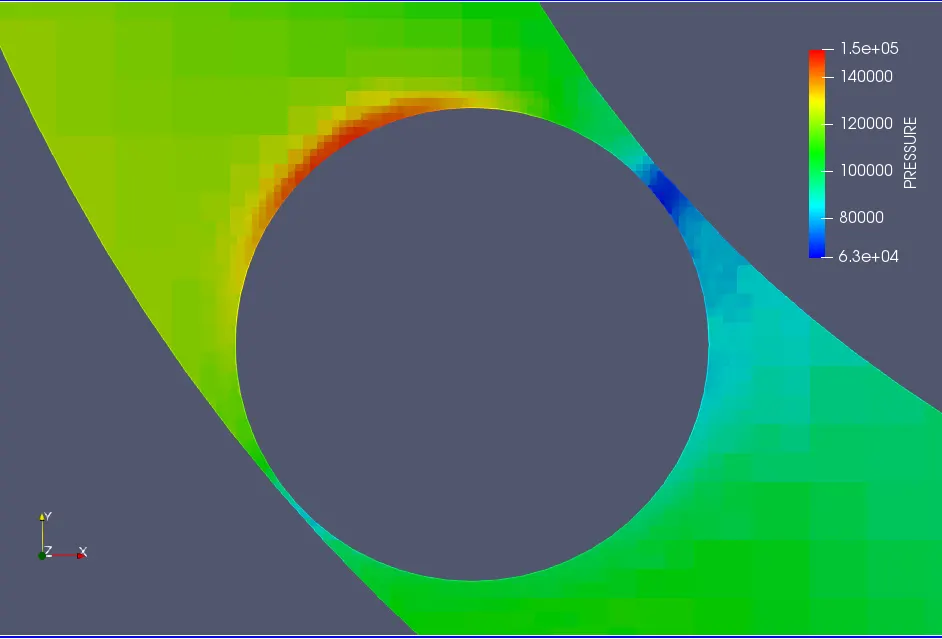
Observation from the Plot:

There are basically two regions which we can see

1. Red Region: This region is the region of high pressure (between 1.4 to 1.5 bar). See how the flowing fluid imposes high pressure on the throttle.

2. Blue region: In this region the pressure is low. The pressure drops because the flow is constricted.

Pressure Contour Plot (at throttle angle = 25 degrees)

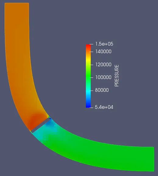
Observation: Pressure drops because of the throttle restricting the flow.

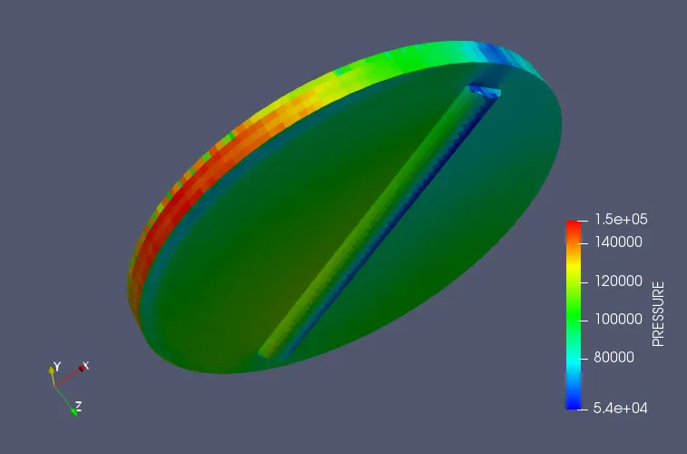
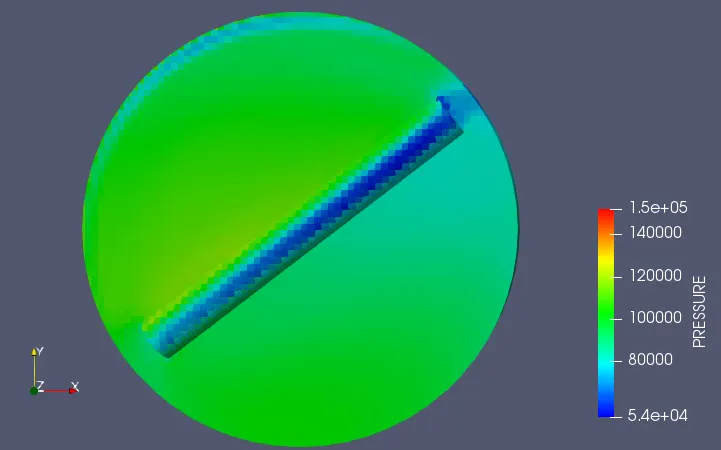
Pressure Contour Plot on the Throttle

Image at Throttle angle = 0 degrees

Observation from the Plot

On the throttle also there are two regions. High pressure and low pressure region. In the red, high pressure region the fluid imposes pressure on the throttle as it flows over the throttle body.

And the low pressure (blue region) is due to the flow separation happening near the axis of rotation (shaft) of the throttle.

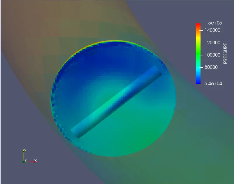
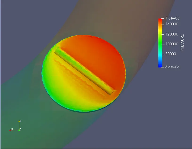
Pressure contour plot at Throttle angle = 25 degrees

1. Throttle side which is facing towards the outlet

2. Throttle side which is facing towards the inlet

Observation from the Plot

On the throttle also there are two regions. High pressure and low pressure region. In the red, high pressure region the fluid imposes pressure on the throttle as it flows over the throttle body.

Throttle side which is facing towards the inlet is at a higher pressure (red face) because it stagnates the flow whereas on the other hand the side which is facing the outlet is at a lower pressure (Blue face) because flow separation happens around the edge of that face.

Velocity Contour Plot

(at throttle angle = 0 degrees)

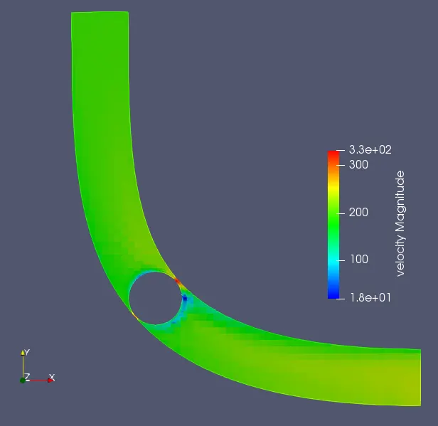
A closer look at the velocity contour plot near the throttle region.

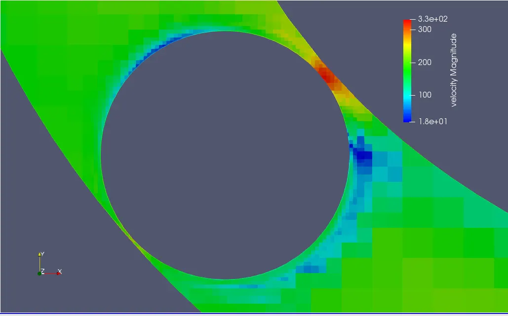
Observation from the above plot:

We can see three regions in the plot.

1. Top left blue region: This is the region before the fluid approaches the throttle. The velocity decreases as the fluid approaches the throttle.

2. Top right red region: In this region the flow area is very small that is why the fluid velocity increases to maintain the mass flow rate. This is the region where the fluid has the maximum velocity. The max velocity goes as high as 330 m/s.

3. Bottom right blue region: This is the recirculation region. Eddies form here and velocity drops to as low as 18 m/s.

Velocity Contour Plot

(at throttle angle = 25 degrees)

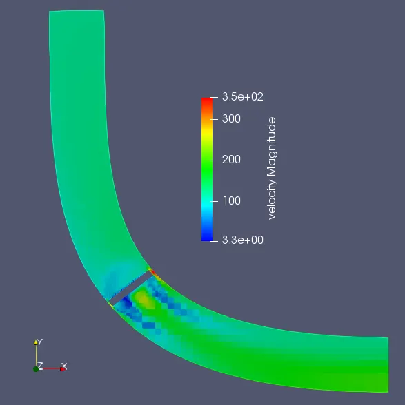
A closer look at the velocity contour plot near the throttle region.

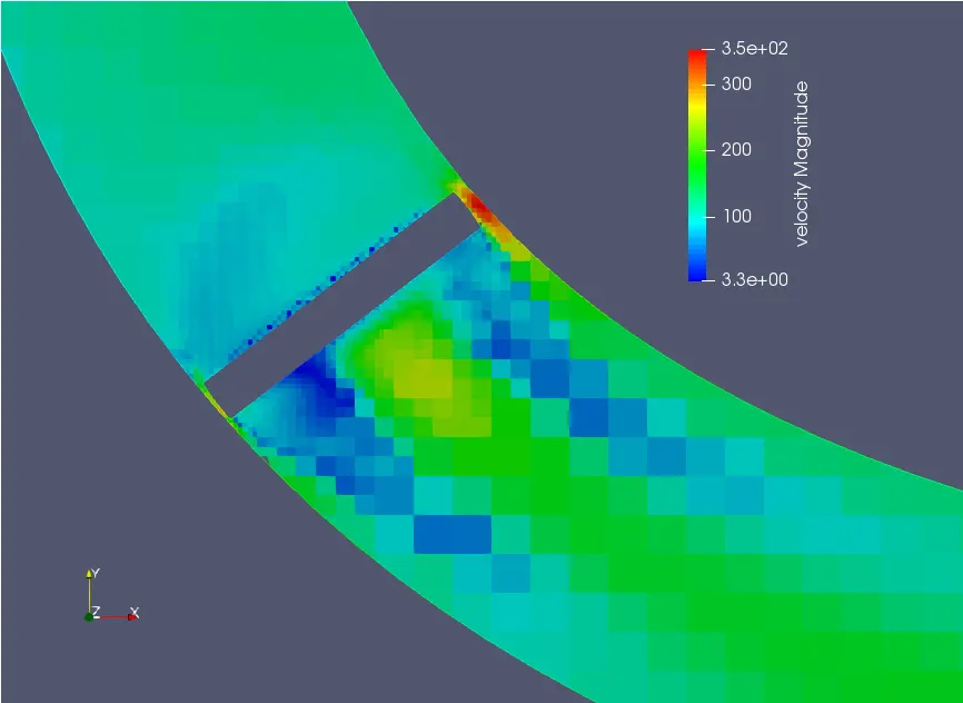
From the above image we can see that flow separation has inreased because the throttle is tilted relative to the flow direction.

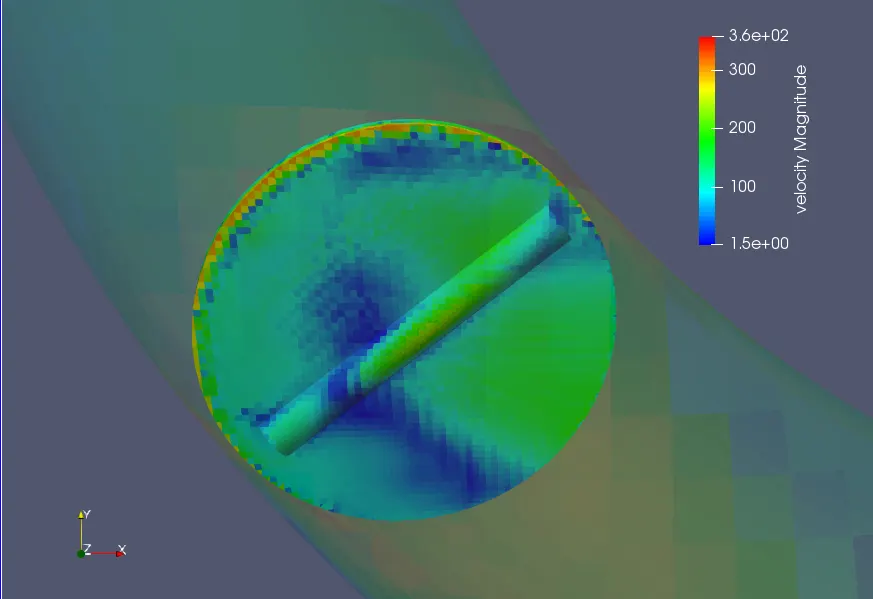
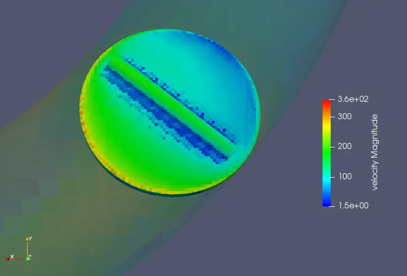
Velocity Contour Plot on the Throttle

Pressure Convergence Plot

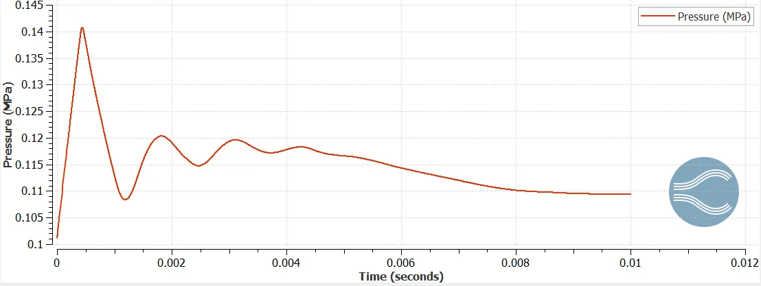
The above plot shows how the pressure fluctuates initially because of the convergence and then because of the rotation of throttle and then becomes steady after 8 milliseconds.

Velocity Convergence Plot

At inlet

At Outlet

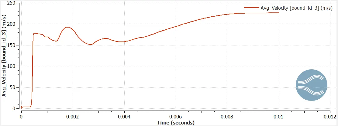
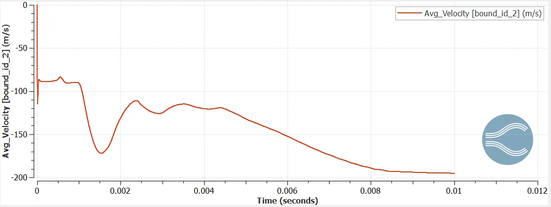
Similar results are obtained for velocity, throttle rotation creates disturbance in the velocity feild both at inlet and outlet boundaries. Velocity becomes stable after the throttle rotation stops at 8 milliseconds.

Mass Flow Rate Plot

Inlet

Outlet

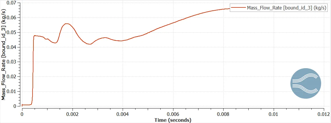
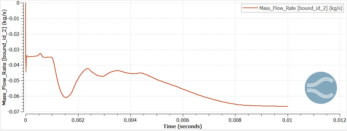
From 4 milliseconds till 8 milliseconds the throttle returns to its original position and reduces the flow restriction and that is why the mass flow rate increases from 4 to 8 milliseconds.

Mass flow rate = 0.066 kg/s

Total Cell Count Plot

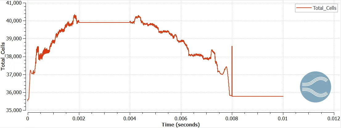
From 0 to 2 milliseconds the throttle rotates from 0 to 25 degrees and since we have used fixed embedding for the throttle the number of mesh cells increases upto and around 40,000. Then from 2 to 4 milliseconds the throttle angle doesn't change so the number of cell count remains the same. Then from 4 to 8 milliseconds the throttle returns to its original angular position (0 degrees) so the number of mesh cells decreases from 40,000 to 35769 cells.

Velocity Animation :

velocity vector field over throttle animation :

Pressure Animation:

Conclusion :

• After observing the above results, it can be concluded that the rotation of the throttle body affects the pressure, velocity and mass flow rate of the flow.
• the mass flow rate of the flow can be controlled by the movement of the throttle body.
• Simulation time is more in the transient case than the one with steady state solver. Refinement of mesh with smaller grid size (2e-3 metres) and fixed embedding made the case setup more complex with greater computational time to solve the problem, The pressure and velocity changes greatly over the throttle body as the throttle moves a certain angle causing a lot of fluctuations over the region.