Genetic Algorithm

1. The algorithm begins by creating a random initial population.

2. Scores each member of the current population by computing its fitness value. These values are called raw fitness scores.

3. Scales the raw fitness scores to convert them into a more usable range of values. These scaled values are called expectation values.

4. Selects members, called parents, based on their expectation.

5. Some of the individuals in the current population that have lower fitness are chosen as elite. These elite individuals are passed to the next population.

6. Produces children from the parents. Children are produced either by making random changes to a single parent—mutation—or by combining the vector entries of a pair of parents—crossover.

7. Replaces the current population with the children to form the next generation.

Code to optimize stalagmite function:

%program to optimise the stalagmite function and find the global maxima of the function.
clear all
close all
clc

%Optimizing  Stalagmite function using genetic algo
x=linspace(0,0.6,150);
y=linspace(0,0.6,150);

%creating meshgrid
[xx yy]=meshgrid(x, y);

%looping

for i=1:length(xx)
    
    for j=1:length(yy)
       
        input_vector(1)=xx(i,j);
        input_vector(2)=yy(i,j);
        f(i,j)=stalgmite(input_vector);
        
    end
    
end

%case1 unbounded values 

iterations=100;

tic
for i=1:iterations
    
    [inputa fval1(i)]=ga(@stalgmite,2);
    x1(i)=inputa(1);
    y1(i)=inputa(2);
    
end
time=toc

%plotting
figure(1)
subplot(2,1,1)
hold on
surfc(x,y,f)
shading interp
plot3(x1,y1,fval1,'marker','*')
title("Case 1 (Unbounded Values)")
subplot(2,1,2)
plot(fval1)
xlabel('No. of Iterations')
ylabel('Function Minimum')

%case 2 (bounding the value of x from 0-1)
%looping
tic
for i=1:iterations
    
    [inputb fval2(i)]=ga(@stalgmite,2,[],[],[],[],[0;0],[1;1]);
    x2(i)=inputb(1);
    y2(i)=inputb(2);
    
end
time2=toc

%plotting
figure(2)
subplot(2,1,1)
hold on
surfc(x,y,f)
shading interp
plot3(x2,y2,fval2,'marker','*')
title("Case 2 (Bounded values)")
subplot(2,1,2)
plot(fval2)
xlabel('No. of Iterations') 
ylabel('Function Minimum')

%case 3 (bounding the values and also increasing the population by 500)

options=optimoptions('ga');
options=optimoptions(options,'populationsize',500)

%looping
tic
for i=1:iterations
    
   [inputc fval3(i)]=ga(@stalgmite,2,[],[],[],[],[0;0],[1;1],[],[],options);
   x3(i)=inputc(1);
   y3(i)=inputc(2);
   
end

time3=toc

%plotting
figure(3)
subplot(2,1,1)
hold on
surfc(x,y,f)
shading interp
plot3(x3,y3,fval3,'marker','*')
title("Case 3 (Increased Population)")
subplot(2,1,2)
plot(fval3)
xlabel('No. of Iterations') 
ylabel('Function Minimum')

Code for Function:

function [F]=stalgmite(input_vector)

x=input_vector(1);
y=input_vector(2);

f1=(sin(5.1*pi.*x+0.5)).^6;
f2=exp(-4*log10(2).*(x-0.0667).^2/0.64);
f3=(sin(5.1*pi*y+0.5))^6;
f4=exp(-4*log10(2).*(y-0.0667).^2/0.64);

F=-f1.*f2.*f3.*f4;

end

Outputs:

Case 1: (Unbounded)

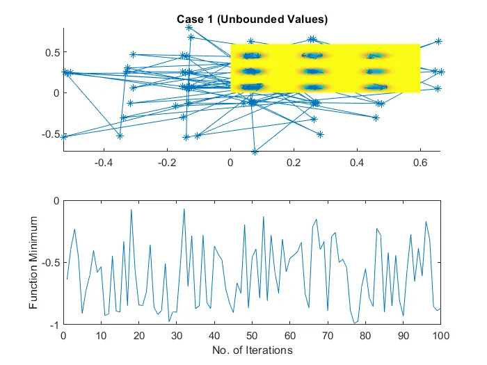
Time is taken = 7.4727 sec

Case 2: Bounded

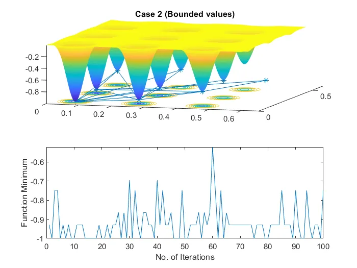
Time is taken = 9.0048 sec

Case 3: bounded with increased population.

Population Size: 500

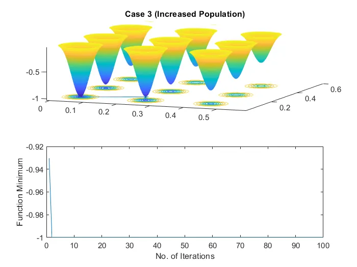
Time is taken = 60.9743 sec