Rankine cycle Simulator

Aim: Create a Rankine Cycle Simulator using OCTAVE/MATLAB.

OBJECTIVE:

• Calculate each state points of the Rankine Cycle (any type of your choice) based on user inputs.
• Plot the corresponding T-s and h-s plots for the given set of inputs.
• Calculate Efficiency.

THEORY:

The Rankine cycle is an idealized thermodynamic cycle of a heat engine that converts heat into mechanical work while undergoing a phase change. It is an idealized cycle in which friction losses in each of the four components are neglected. The heat is supplied externally to a closed loop, which usually uses water as the working fluid.

• Four components of the Rankine cycle:

1. Pump
2. Boiler
3. Turbine
4. Condenser

Governing Equations:

`W_T = m(h_1 -h_2) K`

`Q_r = m(h_2 - h_3) K`

`W_P = m(h_3 -h_4) K`

`Q_b = m(h_1 - h_4) K`

Inputs:

Turbine Inlet temperature = 400° C

Turbine Inlet Pressure = 30 bars

Turbine Outlet Pressure = 0.05 bars = Condenser Inlet Pressure

MATLAB Code:

%Rankine cycle Simulator
%Author: Asad Salah
clear all
clc

% Print Process Description
fprintf('1-2 Isobaric heat Transfern')
fprintf('2-3 Isentropic Expansionn')
fprintf('3-4 Isobaric heat Rejectionn')
fprintf('4-1 Isentropic Compressionn')

%step 1:Enter Inputs
p1 = input('Enter the Pressure at the Turbine Inlet (in bar):');
T1 = input('Enter the Temperature at the Turbineinlet (in Degree Celcius):');
p2 = input('Enter the Pressure at the Condensor (in bar):');

%step 2: Calculate each state point values.
% state point 1
h1 = XSteam('h_pt',p1,T1);
s1 = XSteam('s_pt',p1,T1);

%step 3: state point 2
s2=s1;
sf2 = XSteam('sL_p',p2);
sg2 = XSteam('sV_p',p2);
hf2 = XSteam('hL_p',p2);
hg2 = XSteam('hV_p',p2);   %x2 = (s2-sf2)/(sg2-sf2);
s2 = sg2;
h2 = hg2;                  %hf2 +(x2*(hg2-hf2));
T2=XSteam('T_hs',h2,s2);

%step 4: state point 3
T3=T2;
p3= p2;
s3=XSteam('sL_T',T3);
h3=XSteam('hL_T',T3);
v3 = XSteam('vL_p',p2);

%step 5: state point 4
p4 =p1;
s4= s3;
Cp4 = XSteam('Cp_ps',p4,s4);
Cv4 = XSteam('Cv_ps',p4,s4);
gamma = Cp4/Cv4;
r = (gamma - 1)/gamma;
T4 = T3 *(p4/p3)^r; 

%step 6: Calculate other output values.
Wt = h1-h2;      % Turbine Work      
Wp = v3*(p1-p2)*100;   % Pump Work
h4 = Wp + h3;
W_net = Wt-Wp;     % Net Work unit in kj/kg
Qs = h1 - h4;%heat suppied
N_per = (W_net/Qs)*100;%Efficiency
steam_rate = 3600/(Wt - Wp);%Steam rate per second

%step 7: state point 5 and 6 which help in plotting
T5=XSteam('Tsat_p',p1);
T6=T5;
s5=XSteam('sL_p',p1);
s6=XSteam('sV_p',p1);
h5=XSteam('hL_p',p1);
h6=XSteam('hV_p',p1);

%step 8: print all state poont values to show.
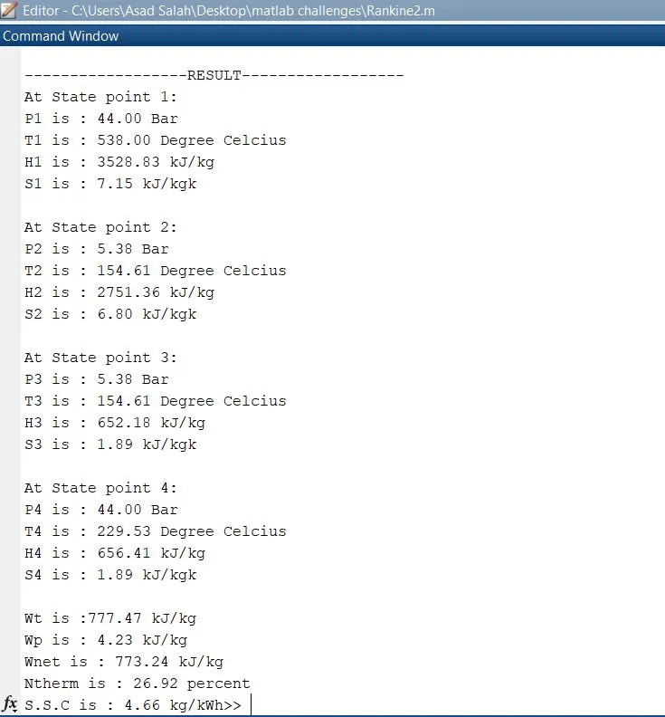
fprintf('n------------------RESULT------------------n')
fprintf('At State point 1:nP1 is : %4.2f BarnT1 is : %4.2f Degree CelciusnH1 is : %4.2f kJ/kgnS1 is : %4.2f kJ/kgknn',p1,T1,h1,s1)
fprintf('At State point 2:nP2 is : %4.2f BarnT2 is : %4.2f Degree CelciusnH2 is : %4.2f kJ/kgnS2 is : %4.2f kJ/kgknn',p2,T2,h2,s2)
fprintf('At State point 3:nP3 is : %4.2f BarnT3 is : %4.2f Degree CelciusnH3 is : %4.2f kJ/kgnS3 is : %4.2f kJ/kgknn',p3,T3,h3,s3)
fprintf('At State point 4:nP4 is : %4.2f BarnT4 is : %4.2f Degree CelciusnH4 is : %4.2f kJ/kgnS4 is : %4.2f kJ/kgknn',p4,T4,h4,s4)
fprintf('Wt is :%4.2f kJ/kgnWp is : %4.2f kJ/kgnWnet is : %4.2f kJ/kgnNtherm is : %4.2f percentnS.S.C is : %4.2f kg/kWh',Wt,Wp,W_net,N_per,steam_rate)

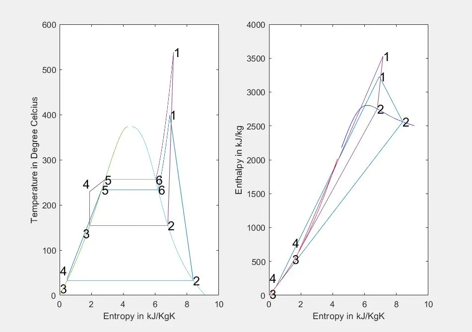
%step 9:plot T-S Diagram
subplot(1,2,1)
T_rankine = linspace(T5,T1,5000);
for i = 1:length(T_rankine)
       s_rankine(i) = XSteam('s_pT',p1,T_rankine(i));
end
plot([s1 s2 s3 s4 s5 s6 s_rankine],[T1 T2 T3 T4 T5 T6 T_rankine]);
hold on
T_curve = linspace(1,400,500);
for i=1:length(T_curve)
    s_l(i) = XSteam('sL_T',T_curve(i));
    s_v(i) = XSteam('sV_T',T_curve(i));
    h_l(i) = XSteam('hL_T',T_curve(i));
    h_v(i) = XSteam('hV_T',T_curve(i));
end
plot(s_l,T_curve);
plot(s_v,T_curve);
text(s1,T1,'1','FontSize',15)
text(s2,T2,'2','FontSize',15)
text(s3,T3,'3','FontSize',15,'HorizontalAlignment','right','VerticalAlignment','top')
text(s4,T4,'4','FontSize',15,'HorizontalAlignment','right','VerticalAlignment','bottom')
text(s5,T5,'5','FontSize',15)
text(s6,T6,'6','FontSize',15)
xlabel('Entropy in kJ/KgK');
ylabel('Temperature in Degree Celcius');

%step 10:plot H-S diagram
subplot(1,2,2)
plot([s1 s2 s3 s4 s1],[h1 h2 h3 h4 h1])
hold on
plot(s_v,h_v,'color','b')
plot(s_l,h_l,'color','r')
text(s1,h1,'1','FontSize',15)
text(s2,h2,'2','FontSize',15)
text(s3,h3,'3','FontSize',15,'HorizontalAlignment','right','VerticalAlignment','top')
text(s4,h4,'4','FontSize',15,'HorizontalAlignment','right','VerticalAlignment','bottom')
xlabel('Entropy in kJ/KgK')
ylabel('Enthalpy in kJ/kg')

Outputs:

Graph:

By-

Asad Salah

(B.E Mechanical)