Week 4 - Genetic Algorithm

Objective

To setup code to optimise the stalagmite function and find the Global maxima of the function.

Theory

Optimisation is a decision making process, it helps to find the best results under a set of prioritized criteria or constraints. It is a procedure which is executed iteratively by comparing various solutions till an optimum or a satisfactory solution is found.

The following is the procedure followed by any optimisation process.

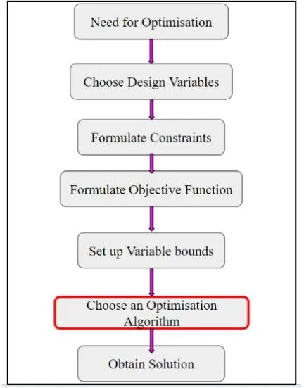
The parameters which you have to vary during the optimisation process are known as variables.

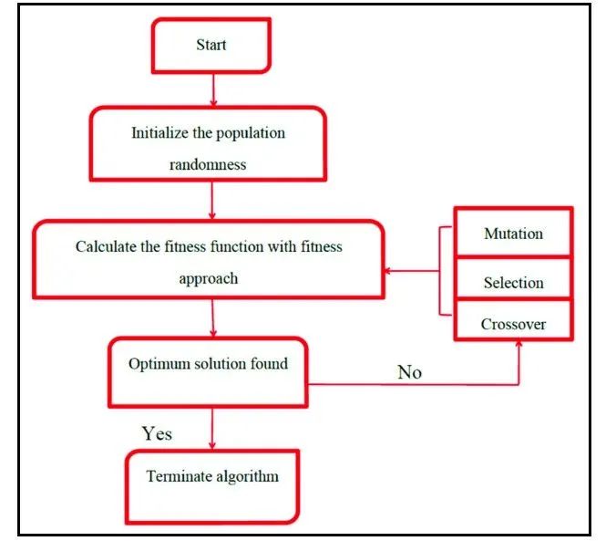
Genetic Algorithm (GA) is a search-based optimization technique based on the principles of Genetics and Natural Selection. It is frequently used to find optimal or near-optimal solutions. It is frequently used to solve optimization problems, in research, and in machine learning.

The following flow chart describes how the genetic algorithm works to find the optimal solution.

Selection

In this step, the parents are selected from the sample data points, the main objective of the selection process is to select the highly fit individuals.

Cross-Over

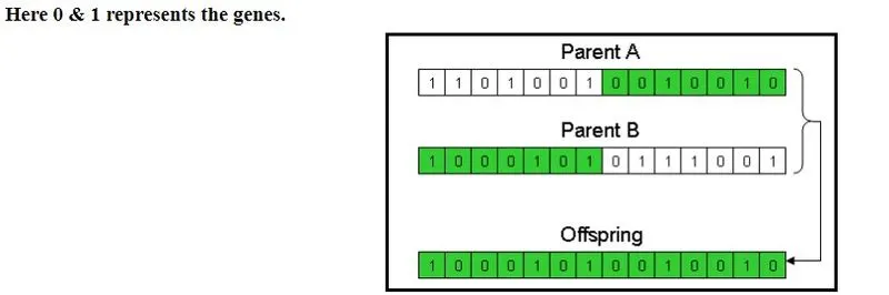
It is the process of taking two parents' solutions and producing the child from them. There are many ways to do cross-over operation, let’s discuss one of the methods. The following method is known as a one-point crossover method, where the set of genes from Parent A is combined with Parent B to create a new offspring.

Mutation

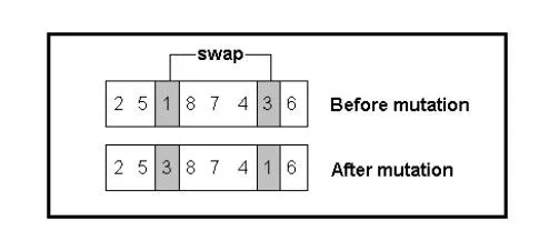
Mutation is carried out to maintain the genetic diversity from one generation of a population of chromosomes to the next. If mutation is not performed, the chromosomes will become too similar to each other, convergence takes place soon and results in local minima.

Similar to the crossover, there are many ways to perform the mutation process.

In these Genetic Algorithm peforms optimisation for a stalagmite function, to find its minima. The stalagmite function has two inputs (x & y) as shown in the figure below.

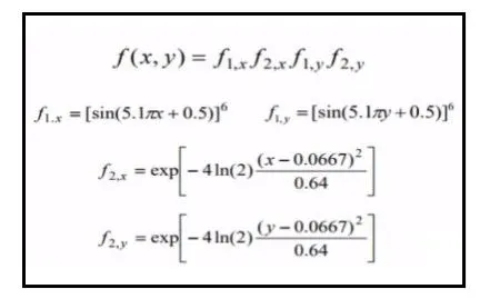
Now, what the fitness function will do is, it will find the value of ‘f’ by varying the sign as well as value of the input arguments(x & y) and find the f-value that should be as minimum as possible. Now, it will compare this fitness value with the optimised value of ‘f’ for every iteration and check how good the fit is.

Main code for 3 studies

clear all
close all
clc

%Defining search space
x = linspace(0,0.6,150);
y = linspace(0,0.6,150);

num_cases=50;


%Creating a 2Dim mesh
[xx yy] = meshgrid(x,y);

%Evaluating the stalagnite function
for i = 1:length(xx)
     for j = 1:length(yy)
          input_vector(1)= xx(i,j);
          input_vector(2)= yy(i,j);
     f(i,j) = stalagmite(input_vector);
     end    
end

%Study : 1 (Unbound inputs)


tic

for a = 1:num_cases
    [input,fopt_1(a)] = ga(@stalagmite,2);
    xopt1(a) = input(1);
    yopt1(a) = input(2);
    
end

study1_time=toc

%Plotting the data
figure(1)
subplot(2,1,1)
hold on
surfc(x,y,-f)
shading interp
colorbar
xlabel('X-axis')
ylabel('Y-axis')
zlabel('Z-axis')

plot3(xopt1,yopt1,-fopt_1,'marker','o','markerfacecolor','r','markersize',5)
title('STUDY 1')
subplot(2,1,2)
plot(-fopt_1)
xlabel('Iterations')
ylabel('Function maxima')

% Study 2 - Statistical behaviour - with upper and lower bounds

tic

for a = 1:num_cases
    [input,fopt_2(a)] = ga(@stalagmite,2,[],[],[],[],[0;0],[0.6;0.6]);
    xopt2(a) = input(1);
    yopt2(a) = input(2);
    
end

study2_time=toc
%Plotting the data
figure(2)
subplot(2,1,1)
hold on
surfc(x,y,-f)
shading interp
colorbar
xlabel('X-axis')
ylabel('Y-axis')
zlabel('Z-axis')

plot3(xopt2,yopt2,-fopt_2,'marker','o','markerfacecolor','r','markersize',5)
title('STUDY 2')
subplot(2,1,2)
plot(-fopt_2)
xlabel('Iterations')
ylabel('Function maxima')


% Study 3 - Statistical behaviour - Increasing GA Iterations

options = optimoptions('ga');
options = optimoptions(options, 'populationsize',250);


tic 
for a = 1:num_cases;
    [inputs,fopt_3(a)]=ga(@stalagmite,2,[],[],[],[],[0;0],[0.6;0.6],[],[],options);
    xopt3(a)=inputs(1);
    yopt3(a)=inputs(2);
end

study3_time=toc
%Plotting the data
figure(3)
subplot(2,1,1)
hold on
surfc(x,y,-f)
shading interp
colorbar
xlabel('X-axis')
ylabel('Y-axis')
zlabel('Z-axis')

plot3(xopt3,yopt3,-fopt_3,'marker','o','markerfacecolor','r','markersize',5)
title('STUDY 3')
subplot(2,1,2)
plot(-fopt_3)
xlabel('Iterations')
ylabel('Function maxima')

disp(-fopt_1)
disp(-fopt_2)
disp(-fopt_3)

Step wise explanation

clear all
close all
clc

%Defining search space
x = linspace(0,0.6,150);
y = linspace(0,0.6,150);

num_cases=50;

%Creating a 2Dim mesh
[xx yy] = meshgrid(x,y);

In these search space for x and y is defined in the range of 0 to 0.6. In these 150 values will be taken for evaluation. All this x and y values are saved in the the mesh grid command which is stored in xx and yy where x values will be in xx and y values will be in yy.

%Evaluating the stalagnite function
for i = 1:length(xx)
     for j = 1:length(yy)
          input_vector(1)= xx(i,j);
          input_vector(2)= yy(i,j);
     f(i,j) = stalagmite(input_vector);
     end    
end

In this commands are used for evaluating the stalagmite function which is defined in the function. The values are calculated from the function . And from the input vector of x and y calculate the position which is stored in i and j. With this position function will setup the value of the function at each position. In xx there will be 150x150 matrix and in yy there will be 150x150 matrix

%Study : 1 (Unbound inputs)

tic

for a = 1:num_cases
    [input,fopt_1(a)] = ga(@stalagmite,2);
    xopt1(a) = input(1);
    yopt1(a) = input(2);
    
end

study1_time=toc

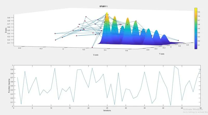
This is the main part of the program in order to get the results for study 1. In these random values will be calculated from above function and get results for study 1

Here the ga function is used to run the stalagmite data and give optimum solution and in the syntax there is number 2 that is nvars (number of design variables). Here there are 2 that is x and y.

tic and toc is used to calculate the total time in order to find the results for these study and which is stored in study1

%Plotting the data
figure(1)
subplot(2,1,1)
hold on
surfc(x,y,-f)
shading interp
colorbar
xlabel('X-axis')
ylabel('Y-axis')
zlabel('Z-axis')
plot3(xopt1,yopt1,-fopt_1,'marker','o','markerfacecolor','r','markersize',5)
title('STUDY 1')
subplot(2,1,2)
plot(-fopt_1)
xlabel('Iterations')
ylabel('Function maxima')

These commands are used to plot the figure

Here the subplot will give Create axes in tiled positions. 2 subplots are defined in order to understand the global minima value from the plot

Colorbar showing color scale

To understand the figure all labels are defined

% Study 2 - Statistical behaviour - with upper and lower bounds

tic

for a = 1:num_cases
    [input,fopt_2(a)] = ga(@stalagmite,2,[],[],[],[],[0;0],[0.6;0.6]);
    xopt2(a) = input(1);
    yopt2(a) = input(2);
    
end

study2_time=toc

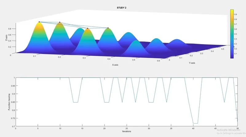
This command is used for the second study. We again perform statistical behaviour with ub and lb i.e upper bounds and lower bounds with some constraint on the solution. UB and LB helps us to improve the optimzation . Consequently its showed us better result form the first case and the points are lowered and iterations is optimizes compared to the first study.

In this to define the upper and lower bounds syntax will be different

x = ga(fun,nvars,A,b,Aeq,beq,lb,ub)

From the command fun is the function name which is given that is stalagmite

nvars is number of design variables

A,b are the Linear inequalities in which in these nothing is there , so it is defined as null by showing [] (square bracket)

Aeq and beq is the linear equalities. In these also nothing is there , so it is defined as null by showing [] (square bracket)

lb and ub is 0 to 0.6

%Plotting the data
figure(2)
subplot(2,1,1)
hold on
surfc(x,y,-f)
shading interp
colorbar
xlabel('X-axis')
ylabel('Y-axis')
zlabel('Z-axis')

plot3(xopt2,yopt2,-fopt_2,'marker','o','markerfacecolor','r','markersize',5)
title('STUDY 2')
subplot(2,1,2)
plot(-fopt_2)
xlabel('Iterations')
ylabel('Function maxima')

These commands are used to plot the figure for study 2

% Study 3 - Statistical behaviour - Increasing GA Iterations

options = optimoptions('ga');
options = optimoptions(options, 'populationsize',250);


tic 
for a = 1:num_cases;
    [inputs,fopt_3(a)]=ga(@stalagmite,2,[],[],[],[],[0;0],[0.6;0.6],[],[],options);
    xopt3(a)=inputs(1);
    yopt3(a)=inputs(2);
end

This are the commands to get the results for study 3.

In these only change is in the change in the syntax of ga. Here in the third study we have another constraint used and known as options as it helps us increase the population to increase the size.

In these we get an exact solution i.e global maxima (a single point) at the top of the function. It is observed that with increase in population size, we get improved convergence, i.e. with higher population, genetic mutation has higher probability to produce offsprings with best genes over a period of time.

Other than that all the function calculation is same.

%Plotting the data
figure(3)
subplot(2,1,1)
hold on
surfc(x,y,-f)
shading interp
colorbar
xlabel('X-axis')
ylabel('Y-axis')
zlabel('Z-axis')

plot3(xopt3,yopt3,-fopt_3,'marker','o','markerfacecolor','r','markersize',5)
title('STUDY 3')
subplot(2,1,2)
plot(-fopt_3)
xlabel('Iterations')
ylabel('Function maxima')

disp(-fopt_1)
disp(-fopt_2)
disp(-fopt_3)

These commands are used to plot the figure for study 3

Function code

function [f] =stalagmite(input_vector)

  x=input_vector(1);
  y=input_vector(2);
  
  f1_x=(sin(5.1*pi*x+0.5))^6;
  f1_y=(sin(5.1*pi*y+0.5))^6;
  
  f2_x=exp(-4*log(2)*((x-0.0667)^2/0.64));
  f2_y=exp(-4*log(2)*((y-0.0667)^2/0.64));
  
  f=-[f1_x*f1_y*f2_x*f2_y];
end

Step wise explanation

These commands are used to define the function. In these the equation is defined in terms of f1_x,f1_y,f2_x and f2_y. From this terms the f value is calculated. This value of f is stored in the function which will go the main code.

Results

Study - 1

Study - 2

Study - 3

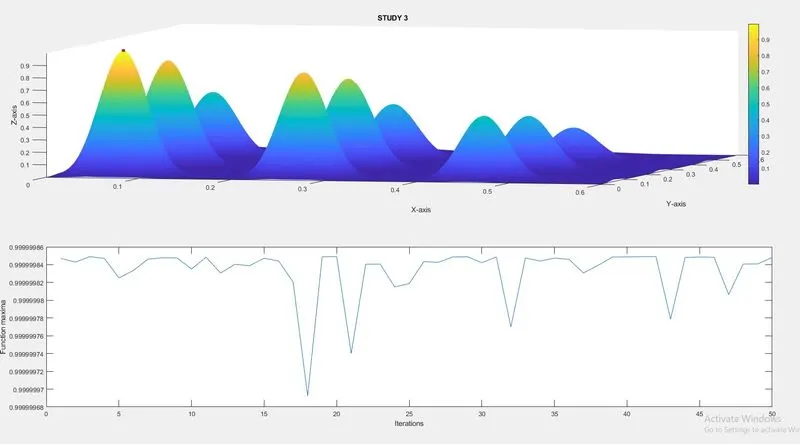
In these case study we will be getting a exact global minima point.

Errors while programming

In these code i just got some error in some spelling errors and the change in variables when assigning the values to plot the figure

For instance in the secong figure for plotting the figure the variable is -fopt_2. But instead of that i used same variable that used in study 1 that is -fopt_1.

Conclusions

In these we have studied Genetic algorithm and learned about the theory of evolution and its importance which helps in prediction of genetic mutation posibilities. Ga in matlab helps us to find the Global minima which helps in engineering level of optimisation for perfect solution and giving the visual context of the solution.