Week 4 - Genetic Algorithm
AIM:
- Write a code in MATLAB to optimise the stalagmite function and find the global maxima of the function.
OBJECTIVE:
- Clearly expalin the concept of genetic algorithm in your own words and also explain the syntax for ga in MATLAB in your report.
- Make sure that your code gives the same output, even if it is made to run several times.
- Plot graphs for all 3 studies and for F maximum vs no. of iterations. Title and axes labels are a must, legends could be shown if necessary.
PROCEDURE:
WHAT IS GA?
Genetic Algorithm (GA) is a search-based optimization technique based on the principles of Genetics and Natural Selection. It is frequently used to find optimal or near-optimal solutions to difficult problems which otherwise would take a lifetime to solve. It is frequently used to solve optimization problems, in research, and in machine learning.
Introduction to Optimization
Optimization is the process of making something better. In any process, we have a set of inputs and a set of outputs as shown in the following figure.
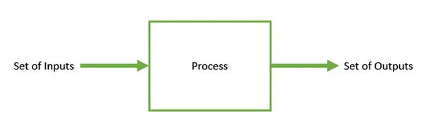
Optimization refers to finding the values of inputs in such a way that we get the “best” output values. The definition of “best” varies from problem to problem, but in mathematical terms, it refers to maximizing or minimizing one or more objective functions, by varying the input parameters.
The set of all possible solutions or values which the inputs can take make up the search space. In this search space, lies a point or a set of points which gives the optimal solution. The aim of optimization is to find that point or set of points in the search space.
Population is a subset of solutions in the current generation. It can also be defined as a set of chromosomes. There are several things to be kept in mind when dealing with GA population −
-
The diversity of the population should be maintained otherwise it might lead to premature convergence.
-
The population size should not be kept very large as it can cause a GA to slow down, while a smaller population might not be enough for a good mating pool. Therefore, an optimal population size needs to be decided by trial and error.
The population is usually defined as a two dimensional array of – size population, size x, chromosome size.
Population Initialization
There are two primary methods to initialize a population in a GA. They are −
-
Random Initialization − Populate the initial population with completely random solutions.
-
Heuristic initialization − Populate the initial population using a known heuristic for the problem.
It has been observed that the entire population should not be initialized using a heuristic, as it can result in the population having similar solutions and very little diversity. It has been experimentally observed that the random solutions are the ones to drive the population to optimality. Therefore, with heuristic initialization, we just seed the population with a couple of good solutions, filling up the rest with random solutions rather than filling the entire population with heuristic based solutions.
It has also been observed that heuristic initialization in some cases, only effects the initial fitness of the population, but in the end, it is the diversity of the solutions which lead to optimality.
Population Models
There are two population models widely in use −
Steady State
In steady state GA, we generate one or two off-springs in each iteration and they replace one or two individuals from the population. A steady state GA is also known as Incremental GA.
GA INBUILD MATLAB COMMANDS ANS SYNTAX
Syntax
Passing Extra Parameters explains how to pass extra parameters to the objective function and nonlinear constraint functions, if necessary.
x = ga(fun,nvars,A,b)x to fun, subject to the linear inequalities A*x ≤ b. ga evaluates the matrix product A*x as if x is transposed (A*x').
x = ga(fun,nvars,A,b,Aeq,beq,lb,ub,nonlcon)nonlcon. The function nonlcon accepts x and returns vectors C and Ceq, representing the nonlinear inequalities and equalities respectively. ga minimizes the fun such that C(x) ≤ 0 and Ceq(x) = 0. (Set lb=[] and ub=[] if no bounds exist.)
x = ga(fun,nvars,A,b,[],[],lb,ub,nonlcon,IntCon)x = ga(fun,nvars,A,b,[],[],lb,ub,nonlcon,IntCon,options)IntCon take integer values.
When there are integer constraints, ga does not accept linear or nonlinear equality constraints, only inequality constraints.
x = ga(problem) finds the minimum for problem, a structure described in problem.
[x,fval] = ga(___), for any previous input arguments, also returns fval, the value of the fitness function at x.
[x,fval,exitflag,output] = ga(___) also returns exitflag, an integer identifying the reason the algorithm terminated, and output, a structure that contains output from each generation and other information about the performance of the algorithm.
[x,fval,exitflag,output,population,scores] = ga(___) also returns a matrix population, whose rows are the final population, and a vector scores, the scores of the final population.
MATLAB CODES FOR all 3 studies and for F maximum vs no. of iterations
clear all
close all
clc

x=linspace(0,0.6,150);
y=linspace(0,0.6,150);

% create 2d mesh
[xx,yy]=meshgrid(x,y);

% evaluate stalagmite function
for i=1:length(xx)
    for j=1:length(yy)
        input_vector(1)=xx(i,j);
        input_vector(2)=yy(i,j);
        f(i,j)=stalagmite_func(input_vector);
    end
end


%surfc(xx, yy, f)


 surfc(xx,yy,-f)
 shading interp

%[x, fval]=ga(@stalagmite_func,2);

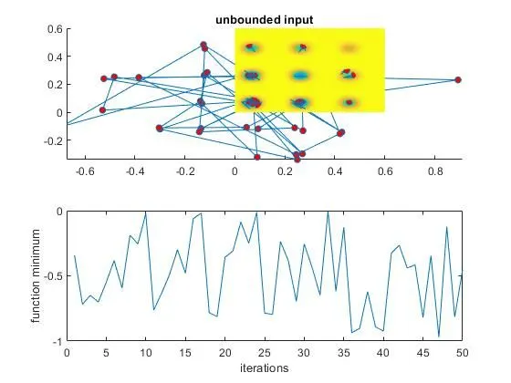
% study 1=statical behaviour
num_case=50;
for i=1:(num_case)
    [input, fopt(i)]=ga(@stalagmite_func,2);
    xopt(i)=input(1);
    yopt(i)=input(2);
end
study1_time=toc
figure(1)
subplot(2,1,1)
hold on
surfc(x, y, f)
shading interp
plot3(xopt,yopt,fopt,'marker','o','markersize',5,'markerfacecolor','r')
title('unbounded input')
subplot(2,1,2)
plot(fopt)
xlabel('iterations')
ylabel('function minimum')

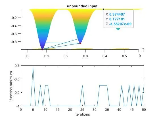
% study_2=upper and lower bound behaviour
for i=1:(num_case)
    [input,fopt(i)]=ga(@stalagmite_func,2,[],[],[],[],[0;0],[0.6;0.6]);
    xopt(i)=input(1);
    yopt(i)=input(2);
end
study2_time=toc
figure(2)
subplot(2,1,1)
hold on
surfc(x, y, f)
shading interp
plot3(xopt,yopt,fopt,'marker','o','markersize',5,'markerfacecolor','r')
title('unbounded input')
subplot(2,1,2)
plot(fopt)
xlabel('iterations')
ylabel('function minimum')

% study_3=boundary vs population
option=optimoptions('ga')
option=optimoptions(option,'populationsize',170)

for i=1:(num_case)
    [input,fopt(i)]=ga(@stalagmite_func,2,[],[],[],[],[0;0],[0.6;0.6],[],[],option);
    xopt(i)=input(1);
    yopt(i)=input(2);
end
study3_time=toc
figure(3)
subplot(2,1,1)
hold on
surfc(x, y, f)
shading interp
plot3(xopt,yopt,fopt,'marker','o','markersize',5,'markerfacecolor','r')
title('unbounded input')
subplot(2,1,2)
plot(fopt)
xlabel('iterations')
ylabel('function minimum')
STALAGMITE FUNCTION:
function [f]=stalagmite_func(input_vector)
x=input_vector(1);
y=input_vector(2);
f1_x=(sin(5.1*pi*x+0.5)).^6;
f2_x=exp((-4)*log(2)*(x-0.0667).^2/0.64);
f1_y=(sin(5.1*pi*y+0.5)).^6;
f2_y=exp((-4)*log(2)*(y-0.0667).^2/0.64);
f=-(f1_x*f2_x*f1_y*f2_y);
end
stalagmite function code:
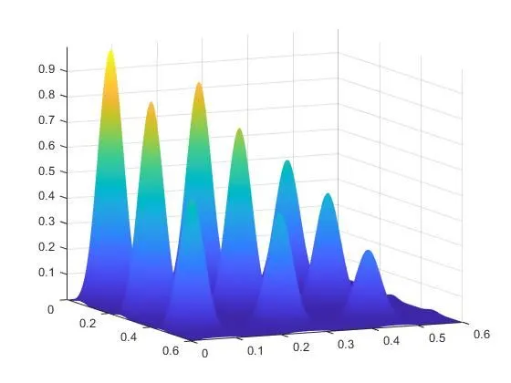
STATICAL BEHAVIOUR:STUDY(1)
UPPER AND LOWER BOUNDARY BEHAVIOUR:STUDY(2)
BOUNDARY WITH POPULATION:STUDY(3)
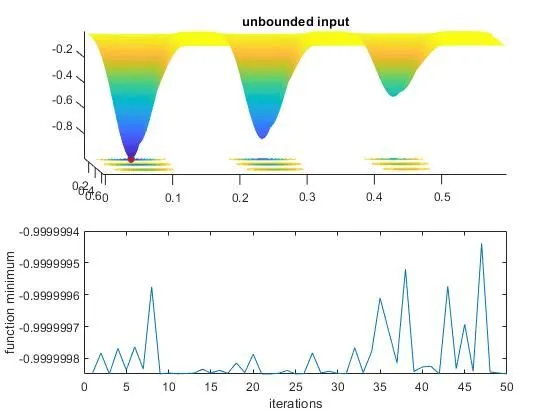
ERROR FACED
STALAGMITE FUNCTION ERROR WHEN CODING
STUDY TIME FOR THREE STUDIES:
study1_time =
7.0460e+03
study2_time =
6.9209e+03
study3_time =
7.0799e+03
conclusion:
therefore genetic algorithm has been codes as per the challenges given in the leaderboard