Week 4 - Genetic Algorithm

Aim: Try to understand the concept of genetic algorithm by referring to varius sources before you attend this challenge. Look out for information regarding stalagmite function and ways to optimise it.

• Write a code in MATLAB to optimise the stalagmite function and find the global maxima of the function.
• Clearly expalin the concept of genetic algorithm in your own words and also explain the syntax for ga in MATLAB in your report.
• Make sure that your code gives the same output, even if it is made to run several times.
• Plot graphs for all 3 studies and for F maximum vs no. of iterations. Title and axes labels are a must, legends could be shown if necessary.

Functions:

t1 = (sin((5.1*pi*x)+0.5))^6

t2 = (sin((5.1*pi*y)+0.5))^6

t3 = exp(((-4)*log(2)*(x-0.0667)^2)/0.64)

t4 = exp(((-4)*log(2)*(y-0.0667)^2)/0.64)

what is ga?

A genetic algorithm (GA) is a method for solving both constrained and unconstrained improvement issues dependent on a characteristic determination measure that imitates natural advancement. The calculation over and again alters a populace of individual arrangements. At each progression, the genetic algorithm haphazardly chooses people from the current populace and utilizations them as guardians to create the kids for the future. Over progressive ages, the populace "develops" toward an ideal arrangement.

You can apply the hereditary calculation to take care of issues that are not appropriate for standard streamlining calculations, remembering issues for which the target work is intermittent, non-differentiable, stochastic, or exceptionally nonlinear.

STALAGMITE FUNCTION

%stalagmite function
function[s_func] = stalagmite(input_vector);
x = input_vector(1)
y = input_vector(2)

t1 = (sin((5.1*pi*x)+0.5))^6;
t2 = (sin((5.1*pi*y)+0.5))^6;
t3 = exp(((-4)*log(2)*(x-0.0667)^2)/0.64);
t4 = exp(((-4)*log(2)*(y-0.0667)^2)/0.64);

s_func = -(t1*t2*t3*t4);
end

MAIN FUNCTION

part1

%define the search space
x = linspace(0,0.6,150);
y = linspace(0,0.6,150);
iterations = 50;

%creating a 2D-mesh
[xx yy] = meshgrid(x,y);

%evaluating the stalagmite function
for i = 1:length(xx);
    for j = 1:length(yy);
        input_vector(1)=xx(i,j);
        input_vector(2)=yy(i,j);
        f(i,j)=s_func(input_vector);
    end
end

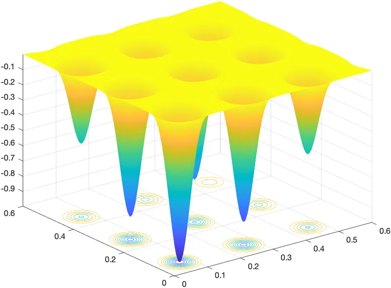
figure(1)
surfc(xx,yy,f)
shading interp

• we have defined search space
• created a 2d mesh using cmd meshgrid
• evaluated the stalagmite function using two for loops.
• created a stalagmite using surfc cmd.

plot for this code:

part2

%study 1 - Statistical Behaviour
tic
for i = 1:iterations;
    [inputs, fval1(i)] = ga(@s_func, 2);
    xval1(i) = inputs(1);
    yval1(i) = inputs(2);
end

study1_time = toc
figure(2)
subplot(2,1,1)
hold on
surfc(x,y,f)
shading interp
plot3(xval1,yval1,fval1,'marker','o','markersize',6,'markeredgecolor','red','markerfacecolor','red')
title('unbound inputs');
subplot(2,1,2)
plot(fval1);
xlabel('iterations');
ylabel('Function Minimum');
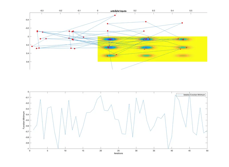
legend('iteration,Function Minimum')

• we have used tic and toc cmd to calculate time taken to solve the function
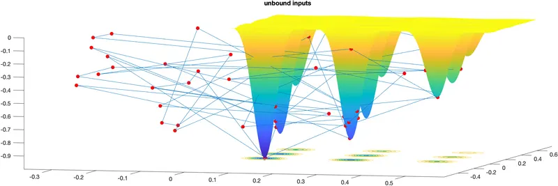
• ga function is called in a for loop which starts from 1 to number of iteration defined. the ga function is responsible for determining the maximum and minimum values in the function
• we have ploted two graphs one containing a 3d stalagmite and second a 2d graph between iteration and minimum values

result : study time = 31.047sec

plot :

part 3

%study 2 - Statistical Behaviour with boundary conditions
tic
for i = 1:iterations
    [inputs1, fval2(i)] = ga(@s_func, 2,[],[],[],[],[0;0],[0.4;0.4]);
    xval2(i) = inputs1(1);
    yval2(i) = inputs1(2);
end

study2_time = toc
figure(3)
subplot(2,1,1)
hold on
surfc(x,y,f)
shading interp
plot3(xval2,yval2,fval2,'marker','o','markersize',6,'markeredgecolor','red','markerfacecolor','red')
title('bounded inputs');
subplot(2,1,2)
plot(fval2);
xlabel('iterations');
ylabel('Function Minimum');
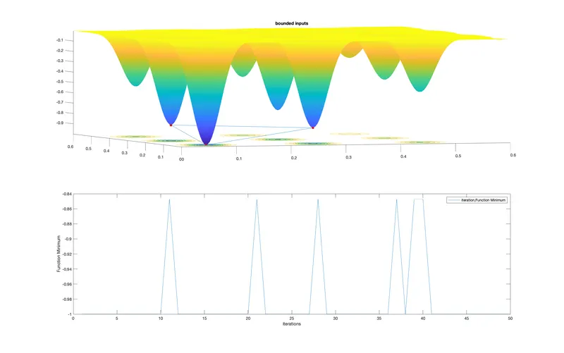
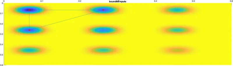
legend('iteration,Function Minimum')

• Similarly like study1, the code remains same but now syntax for ga is different
• here we have added some boundary conditions to narrow our search for the output
• as you can see in study one the value is very stochastic and reading that data is weary so to ease out the data boundary conditions are used

result : study time = 26.52

plot:

part4

%study 3 - Statistical Behaviour with boundary conditions
options = optimoptions('ga','PopulationSize',200)
tic
for i = 1:iterations
    [inputs2, fval3(i)] = ga(@s_func, 2,[],[],[],[],[0;0],[0.4;0.4],[],[options]);
    xval3(i) = inputs2(1);
    yval3(i) = inputs2(2);
end

study3_time = toc
figure(4)
subplot(2,1,1)
hold on
surfc(x,y,f)
shading interp
plot3(xval3,yval3,fval3,'marker','o','markersize',6,'markeredgecolor','red','markerfacecolor','red')
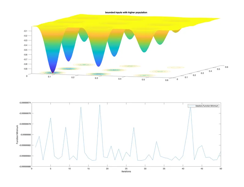
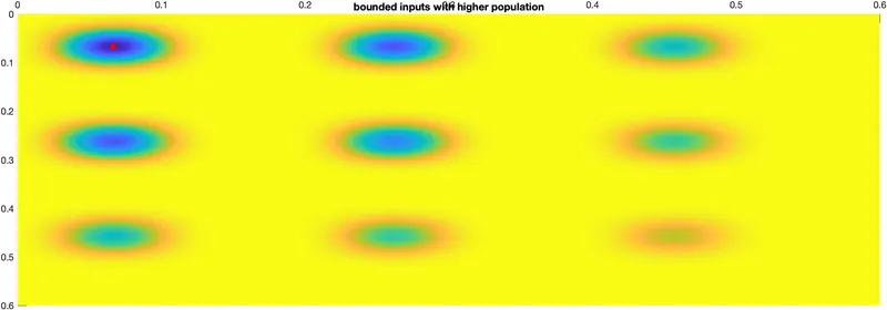
title('bounded inputs with higher population');
subplot(2,1,2)
plot(fval3);
xlabel('iterations');
ylabel('Function Minimum');
legend('iteration,Function Minimum')

• here except ga syntax every code is same as study two
• here we have increased the population by adding options,

plot: