Week 4 - Genetic Algorithm
AIM:
To write a code in MATLAB to optimize the stalagmite function and find the global maxima of the function.
SYNTAX:
Geometric Algorithm-
- x=ga(fun,nvars) where, finds a local unconstrained minimum, x, to the objective function, fun. nvars is the dimension (number of design variables) of fun.
- x =ga(fun,nvars,A,b,[],[],lb,ub,nonlcon,IntCon,options) requires that the variables listed in IntCon take integer values. (Set nonlcon=[] if no nonlinear constraints exist.) lb-Lower bound on x, ub- Upper bound on x
- [x,fval] = ga(___), for any previous input arguments, also returns fval, the value of the fitness function at x.
- Options = optimoptions(solver name, name, value)
Stalagmite Function-
`f(x,y)=f_1x.f_2x.f_1y.f_2y`
Where,
`f_1x=[sin(5.1πx+0.5)]^6`
`f_1y=[sin(5.1πy+0.5)]^6`
`f_2x=exp[-4 log_10(2).(x-0.0667)^2/0.64]`
`f_2y=exp[-4 log_10(2).(y-0.0667)^2/0.64]`
GENETIC ALGORITHM:
Optimization is a decision-making process that is executed iteratively by comparing various solutions to get the optimum/satisfactory solution.
The techniques used are
- Deterministic method
- The output is determined by initial conditions and parameters.
- It follows the stepwise procedure.
- Stochastic method
- It's based on a statistical method, a probabilistic method.
- It’s a predictive model.
Genetic Algorithm is a search-based optimization process to find near to optimal solutions. It is based on random sampling i.e., it starts with a random number of inputs & evaluates the functions based on the inputs. The concept of natural selection occurs where the two genes go under mutation & cross-over to create a better gene.
GA has three important steps determine an optimal fit:
- Selection
- Cross-Over
- Mutation
Selection:
- It involves choosing the highly fit data points as the parent data points from the sample data points.
Cross-Over:
- It is a process of choosing the highly fit parent data from the selection process and producing the next generation from it.
Mutation:
- It is a process of diversifying the population from one generation to the next. Performing mutation is important otherwise the chromosomes will be similar & convergence shall occur.
- Fitness Function is used to find the optimum solution in which the solution is taken as input and how well the solution is suitable to the data is taken as output. It helps determine if the generated gene is optimal for the given data.
- The final stage in the process is terminated, it occurs when the solution generated is close to optimal. Other instances are when the iterations have reached the limit, no change in values for n number of generations when the function has reached its predefined value.
CODE EXPLANATION:
- A search space for the optimization process is created i.e. x & y values created using the ‘linspace’ command to create one-dimensional arrays( i.e. it represents a row or a column index.)
- A 2d mesh is created using the ‘mesh grid’ command(i.e. used to generate x & y matrices for 3-d plots) based on the 1-d arrays.
- The values from the array are nested into an array named ‘input_vector’ which serves as the input to the stalagmite function.
- Surface plots are generated. ‘Shading interp’ command is used to perform shading over the surface plot and to avoid the grid lines.
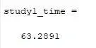
- To show the time taken to run each scenario ‘tic-toc’ command is used.
CODE:
% Defining Boundaries
x = linspace(0,0.6,150);
y = linspace(0,0.6,150);
iterations = 50;

% Generating 2D array
[xx,yy] = meshgrid(x,y);

% Calling Stalagmite function

for i=1:length(xx)
    for j=1:length(yy)
        input_vector(1) = xx(i,j);
        input_vector(2) = yy(i,j);
        f(i,j)= stalagmite(input_vector);
    end
end

figure(1)
surfc(x,y,-f)
xlabel('x value')
ylabel('y value')
title('Stalagmite')
shading interp
OUTPUT:
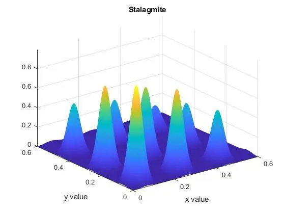
CASE-I:
- Study 1 involves calling the GA function and the upper and lower bounds are not specified.
- [x,fval] = ga(___) syntax is used for calling the stalagmite function. Fopt is the optimum value the function predicts. x contains two inputs(x &y) and there are stored in inputs(1) & inputs(2) respectively.
- A subplot is introduced which helps plot multiple plots inside the same figure window. The surface plot is plotted with the predicted optimum values and another plot where it plots the optimum value according to the iteration is plotted.
CODE:
% Study 1: Statistical Behaviour
for i=1:iterations;
    [inputs,fopt(i)] = ga(@stalagmite,2);
    xopt(i)= inputs(1);
    yopt(i)=inputs(2);
end
study1_time = toc
figure(2)
subplot(2,1,1);
surfc(xx,yy,-f);
hold on
title('Unbounded Stalagmite inputs');
xlabel('x value')
ylabel('y value')
shading interp
plot3(xopt,yopt,-fopt,'marker','o','markersize',5,'markerfacecolor','r')
subplot(2,1,2)
plot(fopt)
xlabel('Iterations')
ylabel('Peak Value')
tic
OUTPUT:
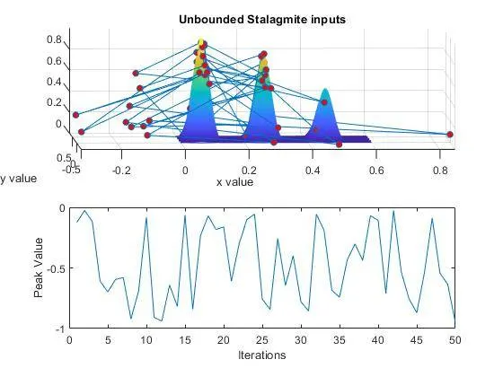
- As it can be seen that the stalagmite function is plotted and the GA is trying to predict the minimum value and it is all over the place due to random sampling. Hence, each time the code is run, a different result occurs. Thus, Case-2 is created.
STUDY TIME:
Case-II:
- Study 2 involves setting upper & lower bounds as the x & y values from case-1 goes below 0 & above 0.6, it is requested to keep it between 0 & 1.
- x =ga(fun,nvars,A,b,[],[],lb,ub,nonlcon,IntCon,options) syntax is used and lower and upper bounds are defined in this function definition.
- The unknown variables in the syntax are disclosed using [] and plots are generated as discussed in case-1.
CODE:
% Study 2: Statistical Behaviour with upper and lower bounds
for i=1:iterations;
    [inputs,fopt(i)] = ga(@stalagmite,2,[],[],[],[],[0;0],[1;1]);
    xopt(i)= inputs(1);
    yopt(i)=inputs(2);
end
study2_time = toc
figure(3)
subplot(2,1,1);
surfc(xx,yy,-f);
hold on
title('Bounded Stalagmite inputs');
xlabel('x value')
ylabel('y value')
shading interp
plot3(xopt,yopt,-fopt,'marker','o','markersize',5,'markerfacecolor','r')
subplot(2,1,2);
plot(fopt)
xlabel('Iterations')
ylabel('Peak Value')
tic
OUTPUT:
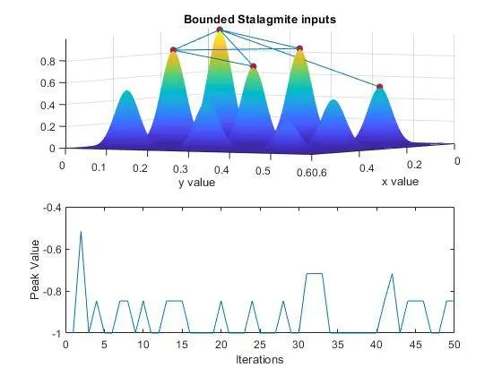
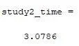
- The function is predicting the maximum point between the 5 peaks. The local maxima is determined but the global maxima could not be generated as the population is very small. Thus, case-3 is created.
STUDY TIME:
Case-III:
The ‘options’ command is used to increase the population size to 170.
CODE:
% Study 3: Increasing GA Iterations
options = optimoptions('ga','PopulationSize',170);
for i=1:iterations;
    [inputs,fopt(i)] = ga(@stalagmite,2,[],[],[],[],[0;0],[1;1],[],[],options);
    xopt(i)= inputs(1);
    yopt(i)= inputs(2);
end
study3_time = toc
figure(4)
subplot(2,1,1);
surfc(xx,yy,-f);
hold on
title('Bounded Stalagmite with increased population size');
xlabel('x value')
ylabel('y value')
shading interp
plot3(xopt,yopt,-fopt,'marker','o','markersize',5,'markerfacecolor','r')
subplot(2,1,2);
plot(fopt)
xlabel('Iterations')
ylabel('Peak Value')
tic
OUTPUT:
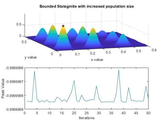
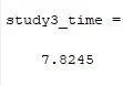
- The drawback of the process is that it takes a lot of time. As the sample size is increased, more individuals are needed to be processed and then to evaluate the function. So, the greater number of iterations will get rid of the problem. Thus, Case-4 is created.
STUDY TIME:
Case-IV:
The population is increased and the inner and outer bound values are decreased for a precise solution.
CODE:
% Study 4: Restricting the Boundary Conditions with increased population size

options = optimoptions('ga','PopulationSize',300);

for i=1:iterations
    [inputs,fopt(i)] = ga(@stalagmite,2,[],[],[],[],[0;0],[0.6;0.6],[],options);
    xopt(i)= inputs(1);
    yopt(i)=inputs(2);
end
study4_time = toc
figure(5)
subplot(2,1,1);
surfc(xx,yy,-f);
hold on
title('Bounded Stalagmite with increased population size and restricted conditions');
xlabel('x value')
ylabel('y value')
shading interp
plot3(xopt,yopt,-fopt,'marker','o','markersize',5,'markerfacecolor','r')
subplot(2,1,2);
plot(fopt)
xlabel('Iterations')
ylabel('Peak Value')
display(inputs) % To display the global maxima x & y values
tic
OUTPUT:
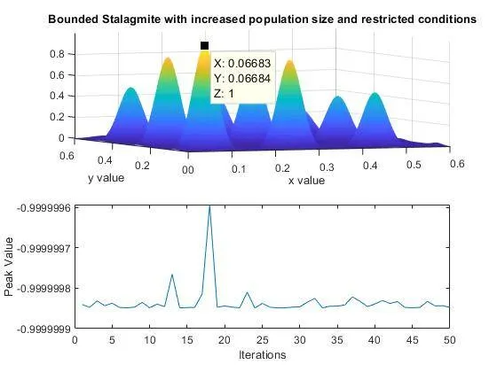
The global maxima is determined and the solution is close to optimal.
Global Maxima is at point(0.06683,0.06684,1)
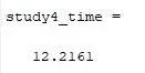
STUDY TIME:
FUNCTION STALAGMITE CODE:
function [f] = stalagmite(input_vector)

x = input_vector(1);
y = input_vector(2);

f1x = (sin(5.1*pi*x+0.5))^6;
f1y = (sin(5.1*pi*y+0.5))^6;

f2x = exp(-4*log(2)*((x-0.0667)^2)/0.64);
f2y = exp(-4*log(2)*((y-0.0667)^2)/0.64);

f = -(f1x*f1y*f2x*f2y);
end
FINAL CODE:
clear all
close all
clc

% Defining Boundaries
x = linspace(0,0.6,150);
y = linspace(0,0.6,150);
iterations = 50;

% Generating 2D array
[xx,yy] = meshgrid(x,y);

% Calling Stalagmite function

for i=1:length(xx)
    for j=1:length(yy)
        input_vector(1) = xx(i,j);
        input_vector(2) = yy(i,j);
        f(i,j)= stalagmite(input_vector);
    end
end

figure(1)
surfc(x,y,-f)
xlabel('x value')
ylabel('y value')
title('Stalagmite')
shading interp

% Study 1: Statistical Behaviour
for i=1:iterations;
    [inputs,fopt(i)] = ga(@stalagmite,2);
    xopt(i)= inputs(1);
    yopt(i)=inputs(2);
end
study1_time = toc
figure(2)
subplot(2,1,1);
surfc(xx,yy,-f);
hold on
title('Unbounded Stalagmite inputs');
xlabel('x value')
ylabel('y value')
shading interp
plot3(xopt,yopt,-fopt,'marker','o','markersize',5,'markerfacecolor','r')
subplot(2,1,2)
plot(fopt)
xlabel('Iterations')
ylabel('Peak Value')
tic

% Study 2: Statistical Behaviour with upper and lower bounds
for i=1:iterations;
    [inputs,fopt(i)] = ga(@stalagmite,2,[],[],[],[],[0;0],[1;1]);
    xopt(i)= inputs(1);
    yopt(i)=inputs(2);
end
study2_time = toc
figure(3)
subplot(2,1,1);
surfc(xx,yy,-f);
hold on
title('Bounded Stalagmite inputs');
xlabel('x value')
ylabel('y value')
shading interp
plot3(xopt,yopt,-fopt,'marker','o','markersize',5,'markerfacecolor','r')
subplot(2,1,2);
plot(fopt)
xlabel('Iterations')
ylabel('Peak Value')
tic

% Study 3: Increasing GA Iterations
options = optimoptions('ga','PopulationSize',170);
for i=1:iterations;
    [inputs,fopt(i)] = ga(@stalagmite,2,[],[],[],[],[0;0],[1;1],[],[],options);
    xopt(i)= inputs(1);
    yopt(i)= inputs(2);
end
study3_time = toc
figure(4)
subplot(2,1,1);
surfc(xx,yy,-f);
hold on
title('Bounded Stalagmite with increased population size');
xlabel('x value')
ylabel('y value')
shading interp
plot3(xopt,yopt,-fopt,'marker','o','markersize',5,'markerfacecolor','r')
subplot(2,1,2);
plot(fopt)
xlabel('Iterations')
ylabel('Peak Value')
tic

% Study 4: Restricting the Boundary Conditions with increased population size

options = optimoptions('ga','PopulationSize',300);

for i=1:iterations
    [inputs,fopt(i)] = ga(@stalagmite,2,[],[],[],[],[0;0],[0.6;0.6],[],options);
    xopt(i)= inputs(1);
    yopt(i)=inputs(2);
end
study4_time = toc
figure(5)
subplot(2,1,1);
surfc(xx,yy,-f);
hold on
title('Bounded Stalagmite with increased population size and restricted conditions');
xlabel('x value')
ylabel('y value')
shading interp
plot3(xopt,yopt,-fopt,'marker','o','markersize',5,'markerfacecolor','r')
subplot(2,1,2);
plot(fopt)
xlabel('Iterations')
ylabel('Peak Value')
display(inputs) % To display the global maxima x & y values
tic
CONCLUSION:
- The Global maxima is generated and printed along with the various case studies and their respective graphs are plotted.
- If the population is too small, the global maxima cant be determined but local maxima can be found.
- Every time GA is run, a different result is generated.
REFERENCES:
https://www.tutorialspoint.com/genetic_algorithms/genetic_algorithms_introduction.htm
https://www.mathworks.com/help/gads/ga.html#d122e41261
https://skill-lync.com/knowledgebase/genetic-algorithm-explained