Week 3 - Solving second order ODEs

AIM:

To solve the second-order ode for the motion of a simple pendulum and simulate the pendulum motion using MATLAB

GOVERNING EQUATION:

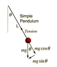
`(d^2 θ)/(dt^2 )+ b/m (dθ)/dt+ g/L sin⁡θ=0` - Eq1

Where

• g is gravity (`m⁄s^2`)
• L is the length of the pendulum (m)
• m is the mass of the ball (kg)
• b is the damping coefficient

DESCRIPTION:

A simple pendulum of mass m and length L is hanging from the point. The pendulum is been displaces to an angle, it will swing back and forth in a periodic motion which can be represented by the above equation by newton’s second law of motion. Solving the equation shall give theta and the rate at which theta changes with respect to time.

In order to solve the equation in MATLAB, the second-order equation is been broken down to simpler ode as follows:

Let`θ= θ_1`

`(dθ)/dt= (dθ_1)/dt= θ_2` - Eq2

`(d^2 θ)/(dt^2 )= d/dt ((dθ_1)/dt)= d/dt (θ_2 )` - Eq3

Sub `θ= θ_1` in Eq1

`(d^2 θ_1)/(dt^2 )+ b/m (dθ_1)/dt+ g/L sin⁡θ_1=0`

Using Eq 2 & 3

`(d^2 θ_2)/(dt^2 )+ b/m (dθ_1)/dt+ g/L sin⁡θ_1=0`

`(dθ_2)/dt= -b/m θ_2 -g/L sin⁡θ_1`

In matrix form,

`d/dt (θ_1|θ_2 )= [(θ_2|-b/m θ_2 -g/L sin⁡θ_1 )]`

`(θ_1¦θ_2 )`is the solution matrix`i.e.`θ`

ODE45 FUNCTION:

Its an inbuilt ode solver in MATLAB.

[t, results] = ode45(@(t,theta)ode_func(t,theta,b,g,l,m),time,theta_0)

Where,

1. Ode is function of t & theta. There are other constants, but t & theta are the dependent and independent functions of ode. @ is the function handler.
2. Ode_func is a separate program in which we define the function. The inputs are b,g,l, and m. The initial conditions are t and theta.
3. Time is the time array i.e. how far the integration is been done is specified using the time array. Theta_0 is the initial condition corresponding to the starting time.

EXPLANATION OF CODE:

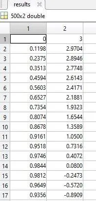
1. The input conditions are given, the solution array containing the angular displacement and angular velocity is shown i.e. 0 and 3, respectively.
2. To integrate the ode system to obtain a solution, the time should be defined, and the limits are provided using the linspace command.
3. The ode function shall define the conversion of the 2^nd order pendulum to a simpler ode. The input arguments with the initial conditions specified are incorporated as mentioned above with eq 2 & 3.
4. The results shall be a column vector i.e. displacement and velocity which is also shown in the output column along with the plots. For verifying the results, the columns will have displacement starting at 0 and the velocity starting at 3, as those were the initial conditions specified while defining the function.
5. The motion of the pendulum is been captured and shown as a movie. Used the movie command to create the animation and the x and y coordinates were calculated using the trigonometric functions.

CODE:

%To simulate the transient behaviour of a simple pendulum.
clear all
close all
clc

%Input conditions
b = 0.05;                  % daming coefficent
g = 9.81;                  % gravity(m/s^2)
l = 1;                     % length of pendulum(m)
m = 1;                     % mass of pendulum(kg)

%Intitial displacement and angular velocity
theta_0 = [0;3];

%Time interval
time = linspace(0,20,500); %time limits

%ODE Solution
[t, results] = ode45(@(t,theta) ode_func(t,theta,b,g,l,m),time,theta_0);

%Plot
figure(1)
plot(t,results(:,1))  %time & angular displacement plot
hold on 
plot(t,results(:,2))  %time & angular velocity plot  
xlabel('time');
ylabel('plot');
grid on;
legend('Angular Displacement & Time', 'Angular velocity & Time')


%Pendulum motion movie
 
 
 for i =1:length(results(:,1))
     
     x0 = 0;
     y0 = 0;
     
     x1 = 1*sin(results(i,1));
     y1 = -1*cos(results(i,1));
     
     figure(2)
     plot([-1,1], [0,0],'linewidth', 3, 'color','r');     
     hold on
     plot([x0 x1], [y0 y1],'linewidth',2,'color','y');
     plot(x1,y1,'o','markersize', 30,'markerfacecolor','b');
     grid on
     axis([-2 2 -2 1.5])
     pause(0.01)
     hold off
     M(i) = getframe(gcf);
         
     
 end
 
 movie(M)
 videofile = VideoWriter('pendulum_animation.avi','uncompressed AVI');
 open(videofile)
 writeVideo(videofile,M)
 close(videofile)

    

The ode_function code:

function [dtheta_dt] = ode_func(t,theta,b,g,l,m)

theta1 = theta(1);
theta2 = theta(2);
dtheta1_dt = theta2;
dtheta2_dt = -(b/m)*theta2 - (g/l)*sin(theta1);
dtheta_dt = [dtheta1_dt; dtheta2_dt];
end

OUTPUT:

The results output showing the displacement and velocity respectively in columns 1 & 2.

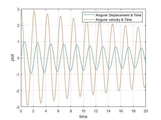
The plot with angular displacement & time, angular velocity & time:

Animation of Pendulum:

https://youtu.be/Zrk3v1MXSKY

ERROR OCCURRED: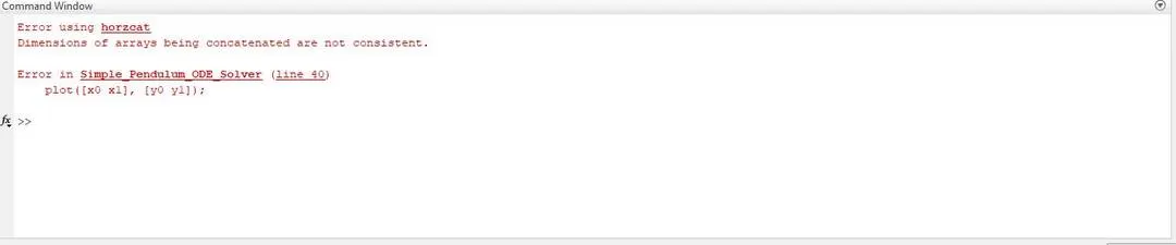

The calculation of x1 and y1 was wrong as it was calculated for the entire row i.e. not using the current value.

ERROR: x1 = 1*sin(results(:,1));

CORRECTION: x1 = 1*sin(results(i,1));

CONCLUSION:

1. The plot between angular displacement and time was created. The plot between angular velocity and time was created and shown. The motion of the pendulum was captured and animated into a movie.
2. The oscillations change when the damping coefficient is changed. If the damping coefficient is changed by a factor of 10, the vibrations can be damped out.