Week 4 - Genetic Algorithm
Genetic Algorithm is a search-based optimization technique based on the principles of Genetic and Natural selection. It is frequently used to find optimal or near-optimal solutions to difficult problems which would take a life-time to solve.
Optimization: Deals with how to minimize or maximize a function.It refers to finding the values of inputs in such way that we get the best output values i.e. maximizing or minimizing one or more obective functions by varying input parameteres.
Syntax:
x = ga(fun,nvars) -> finds a local unconstrained minimum x, to the objective function 'fun'. nvars is the dimension (number of design variables) of fun.
x = ga(fun,nvars,A,b) -> finds a local minimum x,to 'fun', subject to the linear inequalities A*x≤b. ga evaluates the matrix product A*x as if x is transposed (A*x').
x = ga(fun,nvars,A,b,Aeq,Beq) -> finds a local minimum x to 'fun',subect to the linear equalities Aeq*x = beq and A*x≤ b.
x = ga(fun,nvars,A,b,Aeq,Beq,lb,ub) -> defines a set of lower and upper bounds on the design variables.
x = ga(fun,nvars,A,b,Aeq,Beq,lb,ub,nonlcon) -> subjects minimization to the constraints defined in nolcon.
x = ga(fun,nvars,A,b,Aeq,Beq,lb,ub,nonlcon,options) -> minimzes with default optimization parameteres replaced by values in options.
Steps involved:
1) The search space is between 0 to 0.6.
2) The stalagmite function is being called to optimize the function.
3) 'surfc' is used to shade the plot removing lines on it.
4) 'ga' function is used to find the global maximum value in the function.
5) The F output is kept in negative, as 'ga' peaks the minimum value thus b putting negative sign we are reversing the graph plotting so as to get the maximum value easily from the positive output.
CODE:
clear all
close all
clc
%inputs
x = linspace(0,0.6,150);
y = linspace(0,0.6,150);
num_cases = 10;
% meshgrid creation
[xx, yy] = meshgrid(x,y);

% Stalagmite function
for i = 1:length(xx)
    for j = 1:length(yy)
        input_vector(1)=xx(i,j);
        input_vector(2)=yy(i,j);
        f(i,j)= stalagmite_func(input_vector);
    end
end


% Stalagmite function
for i = 1:length(xx)
    for j = 1:length(yy)
        input_vector(1)=xx(i,j);
        input_vector(2)=yy(i,j);
        f(i,j)= stalagmite_func(input_vector);
    end
end

% Study_1 statistical behavior
tic
for i= 1:num_cases
    [inputs,Fopt(i)] = ga(@stalagmite_func,2);
    xopt(i) = inputs(1);
    yopt(i) = inputs(2);
end

study_time_1 = toc;

% Plotting
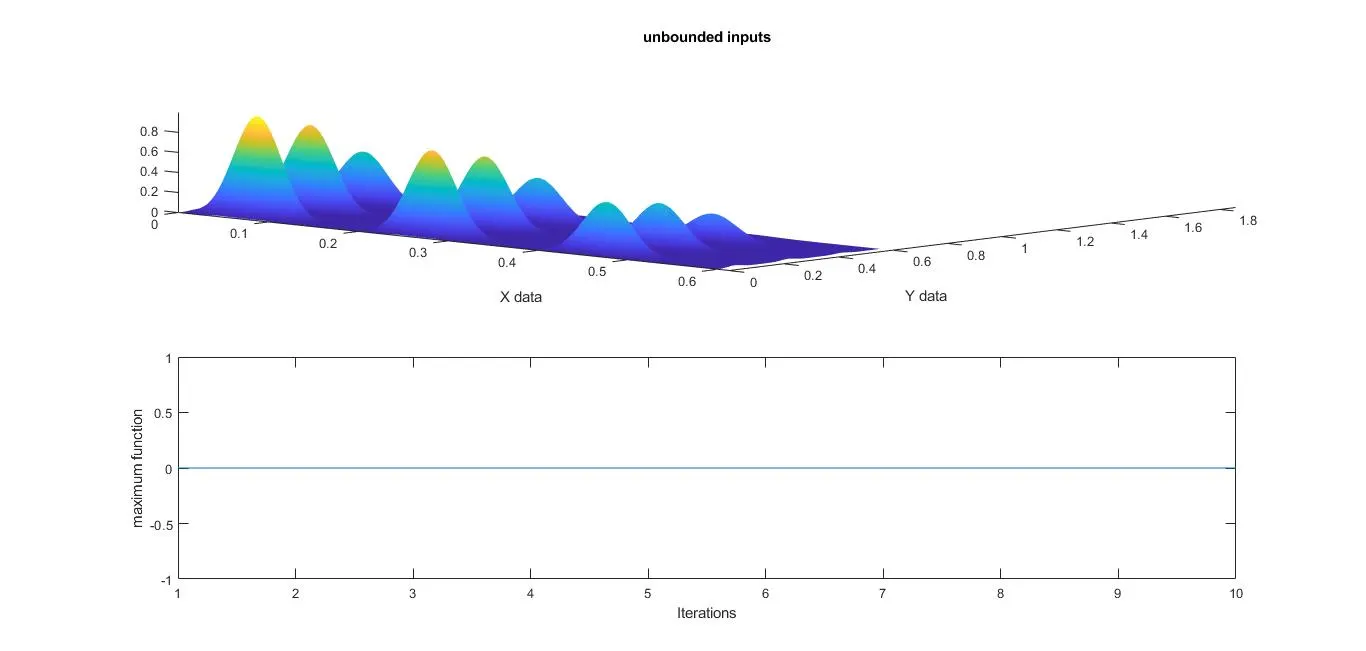
figure(1)
subplot(2,1,1);
hold on
surfc(xx,yy,f);
shading interp;

ylabel('Y data');
xlabel('X data');
plot3(xopt,yopt,Fopt,'marker','o','markersize',5,'markerfacecolor','y')
title('unbounded inputs')
subplot(2,1,2)
plot(Fopt)
xlabel('Iterations')
ylabel('maximum function')

% Study_2 bounded values

tic
for i = 1:num_cases
    [input,Fopt(i)]= ga(@stalagmite_func,2,[],[],[],[],[0;0],[1;1]);
    xopt(i) = inputs(1);
    yopt(i) = inputs(2);
end
study_time_2 = toc;

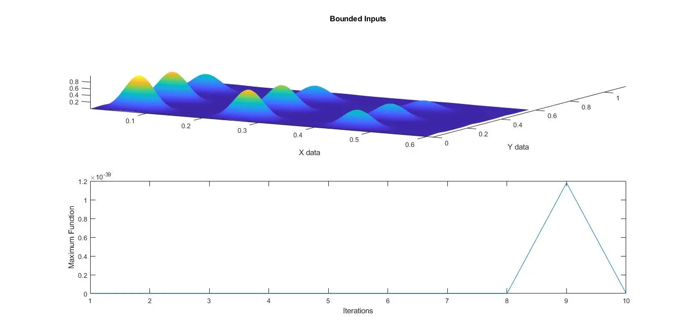
figure(2)
subplot(2,1,1)
hold on
surfc(xx,yy,f)
shading interp
xlabel('X data')
ylabel('Y data')
plot3(xopt,yopt,Fopt,'marker','o','markersize',5,'markerfacecolor','r');
title('Bounded Inputs')
subplot(2,1,2)
plot(Fopt)
xlabel('Iterations')
ylabel('Maximum Function')

% Study_3 bounding the values and increasing population size
options = optimoptions('ga');
options = optimoptions(options,'populationsize',300);
tic
for i = 1:num_cases
    [inputs,Fopt(i)] = ga(@stalagmite_func,2,[],[],[],[],[0;0],[1;1],[],[],options);
    xopt(i) = inputs(1);
    yopt(i) = inputs(2);
end

study_time_3 = toc;

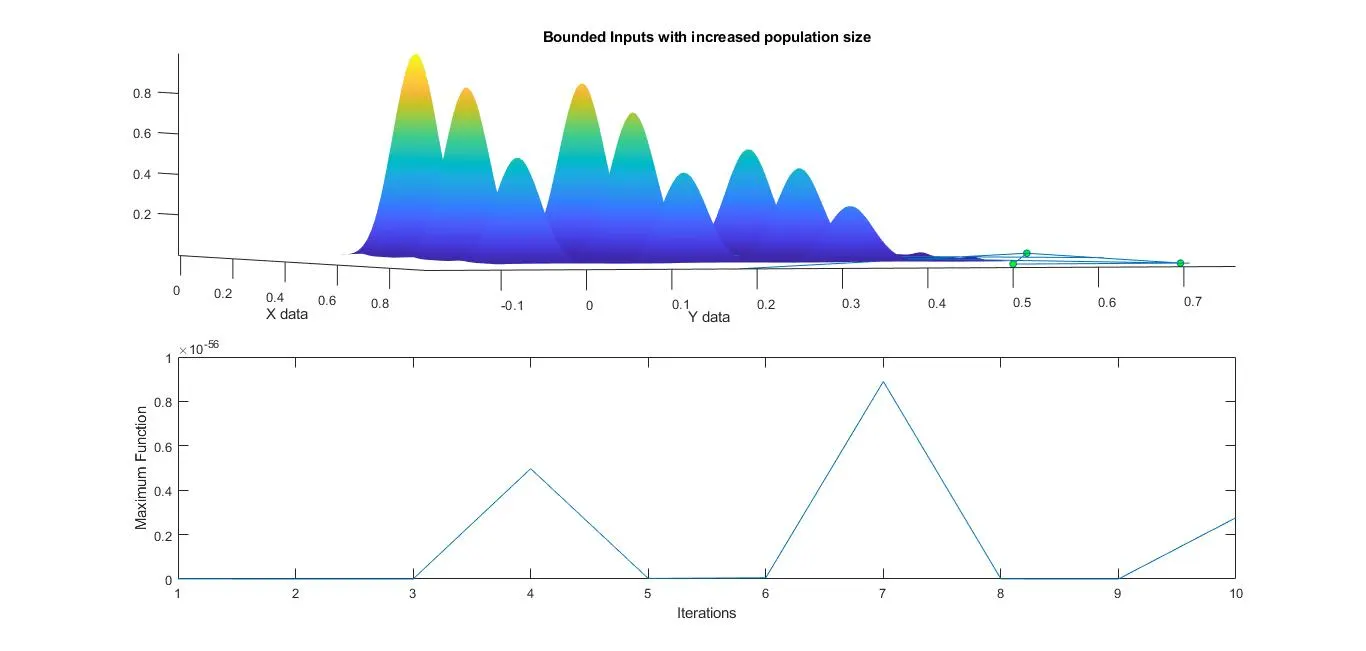
figure(3)
subplot(2,1,1)
hold on
surfc(xx,yy,f)
shading interp
xlabel('X data')
ylabel('Y data')
plot3(xopt,yopt,Fopt,'marker','o','markersize',5,'markerfacecolor','g');
title('Bounded Inputs with increased population size');
subplot(2,1,2)
plot(Fopt)
xlabel('Iterations');
ylabel('Maximum Function');
Stalagmite Function:
function [stalagmite] = stalagmite_func(input_vector)
x = input_vector(1)
y = input_vector(2)
f1_x = (sin(5.1*pi* x + 0.5)).^6;
f2_y = (sin(5.1*pi* y +0.5)).^6;
f3_x = exp((-4*0.6931).*(x-0.0667)^2/(0.64));
f4_y = exp((-4*0.6931).*(y-0.0667)^2/(0.64));
stalagmite = (f1_x.*f2_y.*f3_x.*f4_y)
end
PLOTS:
REFERENCES:
https://www.tutorialspoint.com/genetic_algorithms/genetic_algorithms_introduction.htm