Week 3 - Solving second order ODEs

Aim: To construct a pendulum motion represented by the ODE with damping.

STEPS:

• The 2nd order ODE is solved for obataining first order ODE which can be used in the function 'ode_func'.
• The initial conditons are given.
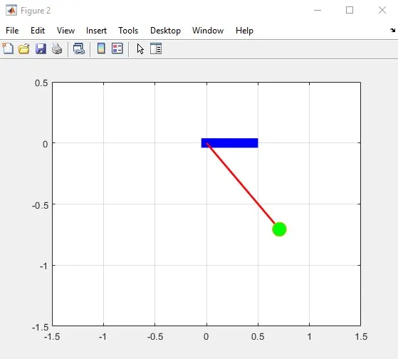
• Image is created for the position of the bob, for every value of t_span.
• Those images are stitched together to make a movie of the pendulum motion.

CODE
function [dtheta_dt] = ode_func(t, theta,b,g ,l ,m)
theta1= theta(1);
theta2= theta(2);
dtheta1_dt = theta(2);
dtheta2_dt = -(b/m)*theta2-(g/l)*sin(theta1);
dtheta_dt = [dtheta1_dt; dtheta2_dt];
end


clear all
close all
clc
%Inputs
b = 0.05;
g = 9.81;
l = 1;
m = 1;
ct = 1;
% Initial condition
disp_v = [0;3];
t_span = linspace(0,20,500);

% ODE
[t,results] = ode45(@(t,theta) ode_func(t,theta,b,g,l,m), t_span, disp_v);

figure(1)
hold on
plot(t,results(:,1))
plot(t,results(:,2))
xlabel('time')
ylabel('plot')
grid on
grid on
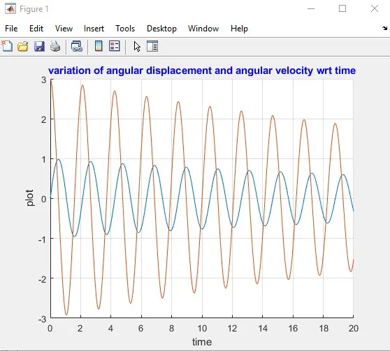
title('variation of angular displacement and angular velocity wrt time','color','b')

theta2 = results(:,1);

for i = 1:length(theta2);
    
    theta_a = theta2(i); % theta _a changes every instant
    x0 = 0;
    y0 = 0;
    
    x1= l*sin(theta_a);
    y1= -l*cos(theta_a);
    % plotting the pendulum
    figure(2)
    plot([-0.05 0.5],[0,0],'color','b','linewidth',10);
    hold on
    plot([x0 x1],[y0 y1],'color','r','linewidth',2);
    hold on
    plot(x1,y1,'o','markers',15,'markerfacecolor','g')
    hold off
    grid on
    axis([-1.5 1.5 -1.5 0.5]);
    pause(0.0003)
    M(ct) = getframe(gcf);
    ct = ct+1;
end
movie(M)
videofile= VideoWriter('pendulum.avi','Uncompressed AVI');
open(videofile)
writeVideo(videofile,M)
close(videofile)

The upper part of the CODE is the ODE function which will be returning values of theta for being used in the main code, for simulating the actual motion of the pendulum.

Figure 1 shows the variation of angular displacement and angular velocity with respect to time.

The figure below shows one image of the video made by MATLAB for depicting the motion of the pendulum.

The link of the youtube video:

https://www.youtube.com/watch?v=tngEve6-c6s