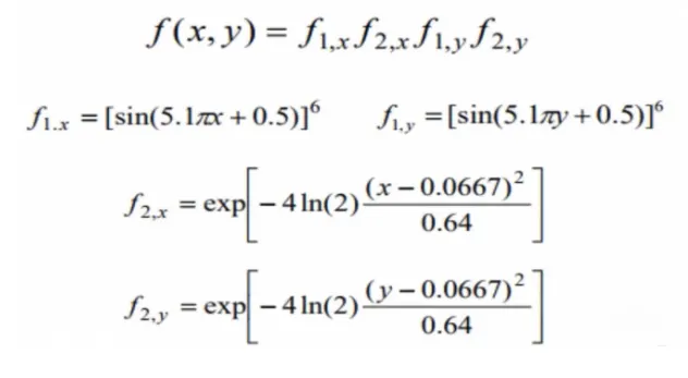
     %%%Write a program to optimize the stalagmite function and find the global maxima
                       with the 'Genetic Algorithm, method.


Objectives:
1.Try to understand the concept of genetic algorithm
2. Write code in MATLAB to optimize the stalagmite function and find the global maxima of the function. explain the concept of genetic algorithm in words and also explain the syntax for ga in MATLAB.


Genetic Algorithm(GA)is an experimental and optimization method introduced by late Charles Darwin also called "Charles Darwin Theory Of evolution". This Algorithm reproduces the process of natural selection where the appropriate individuals are selected for reproduction in order to produce offspring for the next generation.
Phases in GA:
1.	Initialization of Population
The random population of defined size in the code is selected and checked for the fitness of the members where new populations is formed on the basis of the iteration.

2.	Selection
In the selection process, the parents are selected from the data points and the fittest individual are selected and their gens is passed to the next generation. The fitter individual has higher chances of mating and propagating their features to the next generation.

3.	Crossover
It is the process of taking two parent's solutions and producing offspring from them. There are three types in this.
A)	Single point Crossover: A point on both parents chromosomes is picked randomly and designated as “A crossover point’
B)	Two-point: Two points are selected randomly.
C)	Uniform crossover: Each bit is chosen from either parent with equal
         probability.

4.	Mutation
It is performed to maintain genetic diversities from one generation of a population of chromosomes to the next. If not performed the generation will be similar and convergence can take faster.


$$$ Syntax for GA

[ X , Output] = [ func, nvars ,A,b,Aeq,Beq,lb,ub,nonicon,inticon,options]

X = optimum solution
Output = information about optimization process

Func = fitness function
Nvars= No of Variables
A,b = inequality constraint
Aeq,Beq = equality constraint
Lb,ub = Lower imit,Upper lmit
Nonicon = use for nonlinear constraint
Inticon = to get solution in integer
Options = to set population size


-------------------------------------------------------------------------------------
Main Body:

clear all
close all
clc

%Genetic Algorithm problem

x = linspace(0,0.6,150);  %linspace commond is used to define x and y vectors with 150
                          %elements.
y = linspace(0,0.6,150);
%Creaing the 2D mesh grid

[X,Y] = meshgrid(x,y);     % A 2D grid is made using meshgrid where x and y are vectors
                           %specifying the location of grid lines along x and y axes

num_cases = 50;             %Number of itertaion for the problem


for i = 1:length(X)         %For loop is used to solve GA for every element is the grid
    for j = 1:length(Y)
        input_vector(1) = X(i,j);
        input_vector(2) = Y(i,j);
        f(i,j)=stalagmite(input_vector);     %Input vector is declared in the GA where
                                             %each values of mesh frid is stored
    end
end

surfc(X,Y,-f)                                %Genertaing the surface
                                             %Add the labels for x and Y axes witht
                                             %appropriate title.
title('Figure 1. Maximum Function')
xlabel('X value')
ylabel('Y value')
shading interp


-------------------------------------------------------------------------
%%% Statistical behavior without boundation

tic                          %Tic and Toc is used to study the time required in second.

for i=1:num_cases;

%%% To get the optimal values we have GA function with its synatx below.
    [inputs,fopt] = ga(fun,nvars)

inputs represent the values of parameter x and y for which the function has least value(fopt)
fun - the function to be optimized in this case stalagmite
nvars - number of design variables, in our case x and y hence 2.

    [inputs1,fopt1(i)] = ga(@stalagmite,2);
    xopt(i) = inputs1(1);
    yopt (i) = inputs1(2);
end
study1_time = toc;
figure(1)
subplot(2,1,1)        % Subplot commond is used in order plot another plot in same
                       %window
hold on
surfc(X,Y,-f)         %Surface is used to plot the contour for x , y , -f (negative
                      %sign has been introduced for the conveneicence.

xlabel('x value')     %Labelling the plots for three axes
ylabel('y value')
zlabel('function value')
shading interp

%Plot3 is used to plot the 3D plots with various graphics options.

plot3(xopt,yopt,-fopt1,'marker','o','Markersize',4,'markerfacecolor','r')
title('Figure 2.  Statistical Unbound behaviour')

subplot(2,1,2);   %The value of -fopt is plotted in the  second plot second row
plot(-fopt1);
xlabel('iterations');
ylabel('max function');


-----------------------------------------------------------------------------------

%%%%With Upper and Lower limits


tic
for j = 1:num_cases
    [inputs2,fopt2(j)] = ga(@stalagmite,2,[],[],[],[],[0;0],[1;1]);

%Calculating the optimized value of the function at each iteration with limits specified.We have explained the syntax in the introductory part of the code

    xopt1(j) = inputs2(1);
    yopt1(j) = inputs2(2);
end
study2_time =toc;
figure(2)
subplot(2,1,1)
hold on
surfc(X,Y,-f)
shading interp
xlabel('x value')
ylabel('y value')
plot3(xopt1,yopt1,-fopt2,'marker','o','markersize',5,'markerfacecolor','r')
title('Bounded statistical behaviour')
subplot(2,1,2)
plot(-fopt2)
xlabel('iterations')
ylabel('function maximum')


----------------------------------------------------------------------------------------
%%%%%Increse in population


%In this study optimoptions solver is used to solve the problem with the increase in %population. We can work on a large set of numbers where we could find better fitness of the function.

options=optimoptions('ga','PopulationSize',170)

tic
for k=1:num_cases;
    [inputs3,fopt3(k)]=ga(@stalagmite,2,[],[],[],[],[0;0],[1;1],[],[],options);
    xopt(k)=inputs3(1);
    yopt(k)=inputs3(2);
end
study3_time = toc;
figure(3)
subplot(2,1,1)      %The procedure and explanation goes similar to the previous codes
hold on
surfc(X,Y,-f)
xlabel('x value')
ylabel('y label')
zlabel('function value')
shading interp
plot3(xopt,yopt,-fopt3,'marker','o','markersize',5,'markerfacecolor','r');
title('Bounded Statistical Behaviour with Incresed Population Size')
subplot(2,1,2)
plot(-fopt3)
xlabel('iterations')
ylabel('function maximum')


--------------------------------------------------------------------------------------
@@@@@Stalagmite Function
The below fitness function will be used in the main function to find the maxima. We have broken down the equation conveniently with our Input Vector specified.
We have placed a negative sign to reversed the plot and get maxima.

function [f] = stalagmite(input_vector)
x = input_vector(1);
y = input_vector(2);

f1x = (sin(5.1*pi*x + 0.5).^6);
f1y = (sin(5.1*pi*y + 0.5).^6);

t1 = ((x-0.0667).^2)/(0.64);
f2x = exp(-4.*log(2).*t1);

t2 = ((y-0.0667).^2)/(0.64);
f2y = exp(-4.*log(2).*t2);

f = -(f1x.*f2x.*f1y.*f2y);


end
-----------------------------------------------------------------------------
****Problem faced:
The optimooptions solver toolbox was missing and hence unable to execute the code with the current Matlab software which was then solved with the trial version copy.
--------------------------------------------------------------------------------------

####Conclusion
We have successfully demonstrated the GA algorithm to optimize population and have plotted the Bounded,unbounded, and increase in population plots.
This algorithm is boon for the optimization of problems in various applications.