Week 3 - Solving second order ODEs

https://youtu.be/IEKd96vGftA

               

        Write a program to Solve Second Order ODE And Simulate Simple Pendulum


YOUTUBE LINK FOR THE ANIMATION:
https://youtu.be/IEKd96vGft

   The complex static and dynamics motions can be easily performed computationally with mathematical models and functions. One of the major contributors to this is the Ordinary Differential equation(ODE) function. Matlab has provided us a solver that can easily solve complex dynamics problems and demonstrate. 

%%%OBJECTIVES
The objective of the code is to simulate the motion of the pendulum with the help of the Second-order ODE function.
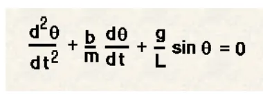
For the simplicity of the problem and for using the Matlab inbuilt ODE45 solver for solving the equation, we will bring down the second-order to the first-order equation.
The equation is shown in the below figure.
This equation is generally a governing equation behind the motion of the pendulum.


ODE 45 solver
(The explanation of the solver is explained in the main code itself for easy demonstration)
The syntax looks something like this.
[t,results] = ode45(@(t,y) ode(t,y,args), tspan, y0)


%%%INPUTS
Damping Coefficients = b= 0.05
aclleration due to gravity = g = 9.81 m/s2
Length of the Pendulum = L1 = 1 meter;
Mass of the bob = m = 0.1 kg 
 Angular Displacment = 0 rad;
 Angular Velocity = 3 rad/sec;

------------------------------------------------------------------------------------
%%%MAIN CODE


clear all
close all
clc


b = 0.05;   %Damping Coefficient
g = 9.81;   %Gravitational Constant
l1 = 1;     %Length of the bob 
m = 0.1;    %Mass of The BOB

%Intial Condition
theta_0 = [0;3]  %intial displacment = 0 and Initial velocity = 3;

%time plots
t_span = linspace(0,20,500);   % Simualting the motion between 0-20 seconds with 
                               % 500 intervals

%Solve ODE


%Another function  has been generated with the name ode_func which has been broken into %first order equation
%(t,theta)it defines the function basically depends on time and theta after that %calling the function and the time span,intial conditions for it.
%(t,results) contains the results that needs to plot for the ode funtion 

[t,results] = ode45(@(t,theta)ode_func(t,theta,b,g,l1,m),t_span,theta_0);


hold on
plot(t,results(:,1))      %plot results(;,1) for angular displacment for the first 
                          %column of the reuslts
hold on
plot(t,results(:,2))      %plot results(;,2) for angular velocity for the second
                          %column of the results

xlabel('Time')            %Labelling the (x,y) axis with Time and Plot
ylabel('Plot')
title('Displacement-Velocity plot');    %Ttitle commond for the plot
legend('Velocity','Displacment');
hold off
grid on

-------------------------------------------------------------------------

ct = 1;                  

for i = 1:length(t)       %%For loop will repeat a statement or a group of 
                          %statments for a fixed no of times.For loop is used to 
                          %generate the possible interval or length
                          %of of t input      
    
    %Intial Points         
                       
    x0 = 0;               %To plot the length and bob of pendulum we will synchronize 
                          %the coordinates with intial postion. As x0=0,Y0=0 as fixed
                          %X1 and Y1 as the length of pendulum 
    y0 = 0;
    x1 = 1*sin(results(i,1));
    y1 = -1*cos(results(i,1));
    
    figure(2)
     %Plotting the length of the bob with line of width 2 with linewidth commond
    plot([x0 x1], [y0 y1],'linewidth',2);       
    hold on
    
    %Plotting pendulum bob with generating the bob of a pendulum with Marker command

    plot(x1,y1,'Marker','O','MarkerSize',20,'MarkerFaceColor','r');
    title('Simulation of Simple Pendulum') 
    
    axis([-1.5 1.5 -1.5 0.5]);    %Setting the axis according to possible results
    pause(0.01)                   
    hold off 
    M(c) = getframe(gcf);         %%To get and store multiple frames, 
                                   %we use array M where "ct" 
                                   %represent individual frames.
                                   %We used getframe commond to get 
                                   %each figure for theta1 and theta2


                                   %ct= i+1 will increment the values 
                                   %accordingly
    ct = ct+1;
    
end

-------------------------------------------------------------------------------------
%Creating a movie

movie(M);                         %To capture all the frames movie command is used. 
                                   %Videowriter command is ued to write the video with 
                                  %its specific name. Also, Open command is used to 
                                   %start video.

videofile = VideoWriter('pendulum.avi', 'Uncompressed avi');
open(videofile)
writeVideo(videofile,M)
close(videofile)
-------------------------------------------------------------------------------------

%%%%%%%%FUNCTION FILE


%To solve this differential equation a separate function file was generated which was %later called into the main program.  

function [ dtheta_dt ] = ode_func( t,theta,b,g,l,m)   

theta1 = theta(1);
theta2 = theta(2);
dtheta1_dt = theta2;
dtheta2_dt = -(b/m)*theta2 - (g/1)*sin(theta1);
dtheta_dt  = [dtheta1_dt; dtheta2_dt];


end
------------------------------------------------------
---------------------------------------------------------------------------------------
%%%%%CONCLUSION and Future Scope
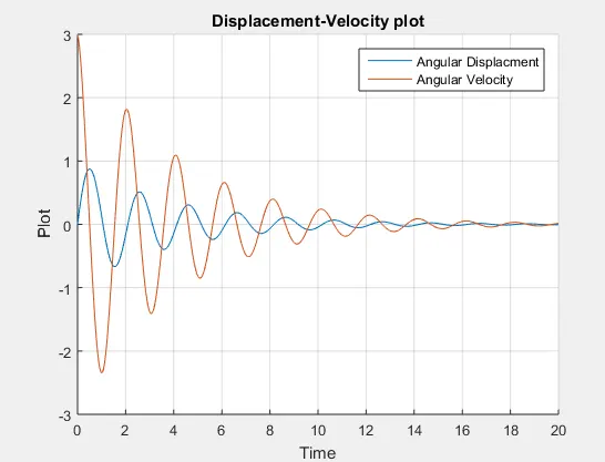
     The Angular velocity and Displacement were successfully plotted with the inputs given in the problem. The animation was generated with the solved ODE function was clearly indicated

***Angular velocity and Displacement decreases due to the damping coefficient which respect to time. One can easily plot the problem with multiple bobs and velocities in the future and easily detonated the dynamics of the motion.