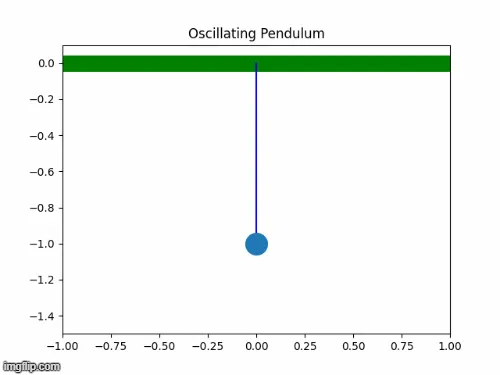
Write a program to Solve Second Order ODE And Simulate Simple Pendulum
            Write a program to Solve Second Order ODE And Simulate Simple Pendulum
                                 using Python.


%%%OBJECTIVES
The objective of the code is to simulate the motion of the pendulum with the help of the Second-order ODE function.
For the simplicity of the problem and for using the Matlab inbuilt ODE45 solver for solving the equation, we will bring down the second-order to the first-order equation.
The equation is shown in the below figure.
This equation is generally a governing equation behind the motion of the pendulum.

In engineering, the ODE is used to describe the transient behaviour of a system.
like we are simulating a simple pendulum problem. The movement of the pendulum
is described by the Newtons second law and when wriiten down we get a second
order differential equation that describes the position of ball with time.

ϴ = Angular Displacement
g  = gravitational accleration
t = time
b = Damping Coefficeint


ODE 45 solver
(The explanation of the solver is explained in the main code itself for easy demonstration)
The syntax looks something like this.
[t,results] = ode45(@(t,y) ode(t,y,args), tspan, y0)


%%%INPUTS
Damping Coefficients = b= 0.05
aclleration due to gravity = g = 9.81 m/s2
Length of the Pendulum = L1 = 1 meter;
Mass of the bob = m = 0.1 kg
 Angular Displacment = 0 rad;
 Angular Velocity = 5 rad/sec;

---------------------------------------------------------------------------------
%%%%MAIN CODE

import numpy as np                     #Import modules for mathematical
                                       #operations,integration and plotting the the
                                       #solved fucntion
from scipy.integrate import odeint
import matplotlib.pyplot as plt
import math

--------------------------------------------------------------------------
#function that returns
def model(theta,t,B,g,l,m):            #Defining the function
	theta1 = theta[0]
	theta2 = theta[1]
	dtheta1_dt = theta2
	dtheta2_dt = -(B/m)*theta2 - (g/l)*math.sin(theta1)
	dtheta_dt = [dtheta1_dt, dtheta2_dt]
	return dtheta_dt
---------------------------------------------------------------------------
B= 0.02
g= 9.81
l= 1
m= 0.1
# Initial condition
theta_0 = [0,5]           %intial displacment = 0 and Initial velocity = 5 rad/sec;

#Time Points
t = np.linspace(0,10,200)  %Defining array 't'for simulating pendulum between 0-10 sec
                           %with 200 points values in between.

#Solve ode
theta = odeint(model,theta_0,t,args = (B,g,l,m))


#Plot results
plt.figure()

plt.plot(t,theta[:,0],'b',label=r'Angular Displacement') %plotting the results(;,1) for
                                                         %angular displacment
plt.plot(t,theta[:,1],'r',label=r'Angular Velocity') %plot results(;,2) for angular
                                                     %velocity

plt.xlabel('Plot')            %Labelling the (x,y) axis with Time and Plot
plt.ylabel('Time')
plt.legend(loc='best')
plt.show()


#Plotting and generating the bob
X0 = 0                            %To plot the length and bob of pendulum we will
                                  %synchronizethe coordinates with intial position
                                  % As x0=0,Y0=0 as fixed
                                  %X1 and Y1 as the length of pendulum
Y0 = 0
ct=1
for i in theta[:,0]:

	X1 = 1*math.sin(i)
	Y1 = -1*math.cos(i)
	filename =  str(ct) + '.png'
	ct = ct + 1               %ct= i+1 will increment the values

	plt.figure()
	plt.plot([-1,1],[0,0],"green",linewidth=15)
	plt.plot([X0,X1],[Y0,Y1],'b-')
	plt.xlim([-1,1])         %Setting the axis according to possible results.
	plt.ylim([-1.5,0.1])

#Plotting the length of the pendulum bob with generating the bob of a pendulum with Marker command
	plt.plot(X1,Y1,marker='o', markersize=20)
	plt.title('Oscillating Pendulum')
	#plt.savefig(filename)


--------------------------------------------------------------------------------
%%%%%CONCLUSION and Future Scope
     The Angular velocity and Displacement were successfully plotted with the inputs given in the problem. The animation was generated with the solved ODE function was clearly indicated

***Angular velocity and Displacement decreases due to the damping coefficient which respect to time. One can easily plot the problem with multiple bobs and velocities in the future and easily detonated the dynamics of the motion.

#https://imgflip.com/gif/4s159u