Optimization using Genetic Algorithm

Aim

To optimise a stalagmite function and to find its maxima

Objectives

Here we have to understand the concept of genetic algorithm and stalagmite unction. Then we must prepare a code to optimise the stalagmite and find its global maxima.

Theories

Genetic Algorithm

We all know about the biological evolution and the phenomenon known as natural selection put forward by Mr. Charles Darwin. There are constrained and unconstrained problems in these theories. We use the optimization technique to solve it. Genetic algorithm is a method that we generally use. It repeatedly modifies a selected population of individual solutions.

At each step, genetic algorithm selects random individuals and predicts the next generation. Over successive generation, the population reaches optimized condition. We can apply the concept of genetic algorithm in any mixed or complicated function to optimize it.

The specialities of genetic algorithm from classical algorithm are listed below,

1. It creates a population of points at each iteration and the best point will be chosen for optimal solution.
2. It selects the next generation by computations which uses random number generations.

The basic steps of a genetic algorithm are represented below,

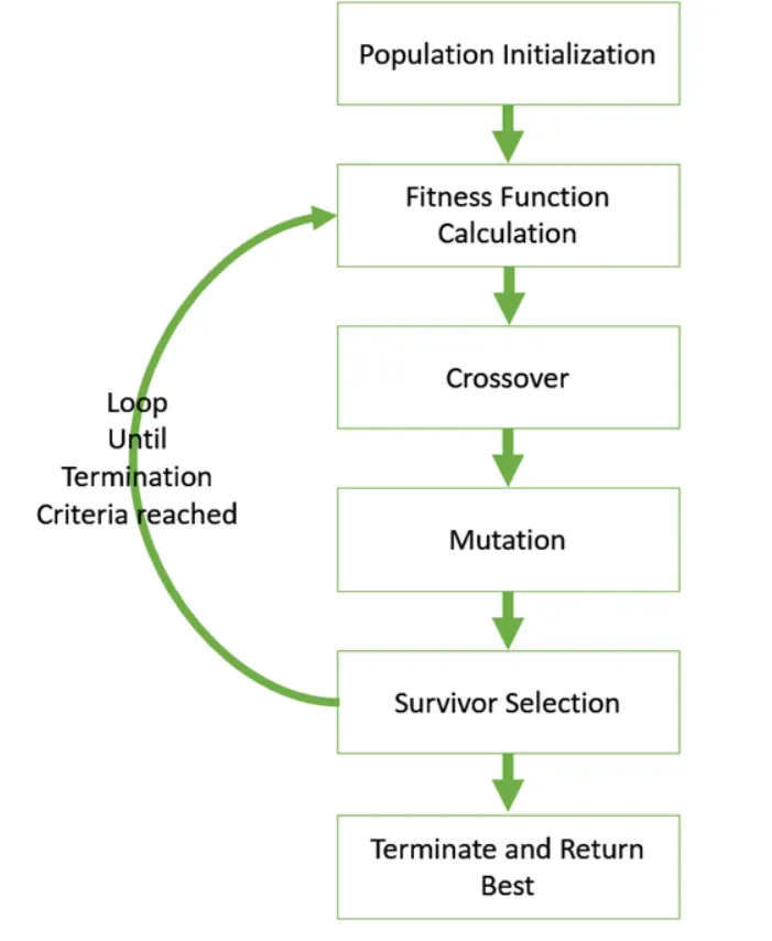
Population initialization begins with a set of individuals. Each individual is characterized by set of parameters.

Fitness function calculation determines, how fit an individual compared to others then individuals will get selected on the basis of score got from fitness function.

For each pair of parents, crossover point is chosen at random. Some offspring’s will show mutation. Finally the best survivor is selected.

Syntax of ga

x = ga(problem) finds the minimum for problem, were problem is a structure

[x,fval] = ga(__) fo any previous input arguments, also returns fval, the values of the fitness function at x

generally,

[x,fval] = ga(fun,nvars,A,b,Aeq,beq,LB,UB,nonlcon,intcon,options)

x is the local unconstrained minimum

fun is objective function

nvars is the number of design variables

A,b is the linear inequalities A*x < or = b

Aeq,beq is the linear inequalities Aeq*x < or = beq

LB and UB sets the lower and upper bound for genetic algorithm

nonlcon and intcon sets non linear and integer the constrains for ga

options allow to add extra parameters.

References : https://in.mathworks.com/help/gads/what-is-the-genetic-algorithm.html

https://www.tutorialspoint.com/genetic_algorithms/genetic_algorithms_fundamentals.htm

Stalagmite

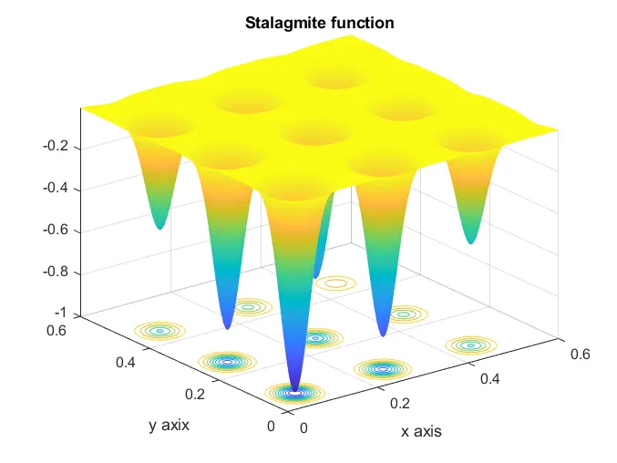
Stalactites and Stalagmite are the pointed icicle type formation seen in natural caves due to mineral depositions. A stalagmite is an upward growing mound of mineral deposits. So stalagmite function is a mathematical function which has the shape of a stalagmite.

Reference : https://oceanexplorer.noaa.gov/facts/stalactite.html#:~:text=A stalagmite is an upward,mineral formations found in caves.

Considering the equation,

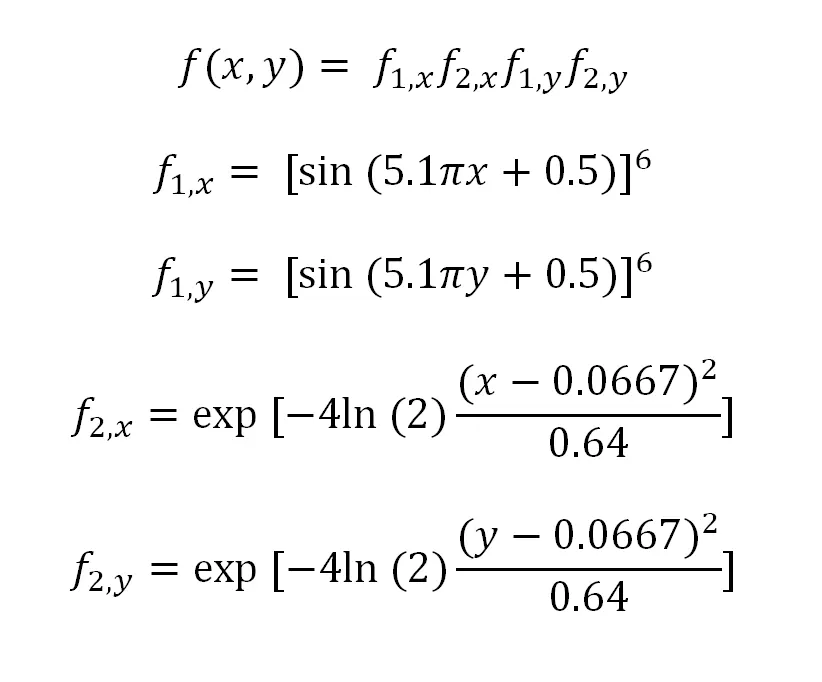
This equation is used to create the programme for stalagmite function

Code for stalagmite function

function[inputs] = stalagmite(input_vector)
x1 = input_vector(1);
y1 = input_vector(2);

f1_x = (sin(5.1*pi*x1+0.5))^6;
f1_y = (sin(5.1*pi*y1+0.5))^6;

f2_x = exp(-4*log(2)*(x1-0.0667)^2/0.64);
f2_y = exp(-4*log(2)*(y1-0.0667)^2/0.64);

[inputs] = -(f1_x*f1_y*f2_x*f2_y);
end

Explanation

Here, we are giving input parameters for the equation in each term and the final result is calculated in f

-f is used to get the value for maxima.

With this function programe,we will work on the optimization programme.

Code

close all
clear all
clc

% Defining search space
x = linspace(0,0.6,150);
y = linspace(0,0.6,150);
[xx yy] = meshgrid(x,y);

% Evaluating stalagmite function
for i = 1:length(xx)
    for j = 1:length(yy)
        input_vector(1) = xx(i,j);
        input_vector(2) = yy(i,j);
        f(i,j) = stalagmite(input_vector);
    end
end

% Ploting Stalagmite Function
surfc(xx,yy,f)
xlabel('x axis')
ylabel('y axix')
shading interp
[inputs,fval] = ga(@stalagmite,2);
title('Stalagmite function')

num_cases = 50;

% Study 1 - Statistical behaviour
tic
for i = 1:num_cases
    [inputs,fopt(i)] = ga(@stalagmite,2);
    xopt(i) = inputs(1);
    yopt(i) = inputs(2);
end
study_time1 = toc

% Plotting Study 1
figure(1)
subplot(2,1,1)
hold on
surfc(x, y, f)
shading interp
plot3(xopt,yopt,fopt,'marker','o','markersize',5,'markerfacecolor','r')
title('Unbounded Inputs')
subplot(2,1,2)
plot(fopt)
xlabel('Iterations')
ylabel('Function Maximum')

% Study 2 - With upper and lower bounds
tic
for i = 1:num_cases
    [inputs,fopt(i)] = ga(@stalagmite,2,[],[],[],[],[0,0],[1,1]);
    xopt(i) = inputs(1);
    yopt(i) = inputs(2);
end
study_time2 = toc

% Plotting Sudy 2
figure(2)
subplot(2,1,1)
hold on
surfc(x, y, f)
shading interp
plot3(xopt,yopt,fopt,'marker','o','markersize',5,'markerfacecolor','r')
title('Bounded Inputs')
subplot(2,1,2)
plot(fopt)
xlabel('Iterations')
ylabel('Function Maximum')

% Study 3 - Increasing GA iterations

options = optimoptions('ga');
options = optimoptions(options,'PopulationSize',170)

tic
for i = 1:num_cases
    [inputs,fopt(i)] = ga(@stalagmite,2,[],[],[],[],[0,0],[1,1],[],[],options);
    xopt(i) = inputs(1);
    yopt(i) = inputs(2);
end
study_time3 = toc

% Plotting Study 3
figure(3)
subplot(2,1,1)
hold on
surfc(x, y, f)
shading interp
plot3(xopt,yopt,fopt,'marker','o','markersize',5,'markerfacecolor','r')
title('Bounded With Increased Population')
subplot(2,1,2)
plot(fopt)
xlabel('Iterations')
ylabel('Function Maximum')

Explanation

The code can be classified in to four parts. They are Calculation of stalagmite, Unbounded condition, Bounded study and study with increased population size.

Previously, we created the function programme for stalagmite. In the first section, that function is used to evaluate the stalagmite function with a defined search space. Then the results are commanded to plot.

But here e need a clear result for the ga. So to get the maxima of ga, the next part of the code was written. Here the number of cases were provided and unbounded inputs were plotted. To get moe correct result the study 2 and 3 were conducted. In study 3 , the population size was increased so that iterated values can be more clear

Results

The outputs are

Unbounded Inputs (Study 1)

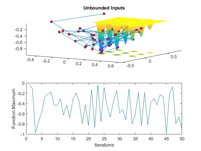
Explanation of plot

Here, the ga values are wrong and they are very much random. So we do the second study. From the iterations, ga values change rapidly and no constant value is showing.

Bounded Inputs (Study 2)

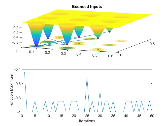
Explanation of plot

Here, the results are more arranged than the previous study. But still not correct. So we do the third study we will increase the population size

Bounded inputs with increased population size (Study 3)

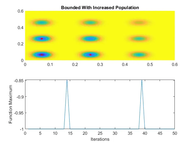
Explanation of plot

From the plot it is clear that, only two times the iteration value is changing. Otherwise it is having constant value. Even if it is changing, it is only oscilatting in a small interval. If we increase the population size further, we can achieve more small interval.

Conclusion

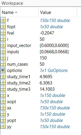
Study time for the programe is given in the workspace. Each time we run the programe, the result will get change. Because ga select the values randomly.

By succesive study the global maxima of the stalagmite function is found which is 1