Week 4 - Genetic Algorithm
Genetic Algorithm :-
Genetic Algorithm is used to find the solutions to optimisation and search problems by effecaciously applying the concept of mutation, crossover and selection.
In GA(Genetic Algorithm), a better solution is accounted by the dynamic evolution of a population of candidate solutions.
How genetic algorithm works:-
In each generation, the fitness value is calculated with population beginning from randomly generated individuals in iteration. More fit individuals in the elitist group are randomly selected from the existing population and each individual genome is recombined and also mutated rendering the formation of a new generation. The new generation is then used for the next iteration. Termination occurs when a satisfactory level has been reached for the population or a maximum number of generations has been produced.
A genetic algorithm requires genetic representation and fitness function definition. Once the fitness function and the genetic representation are defined, the algorithm proceeds for initialization.
Pretty much often is the population generated randomly, this is called initialization. Next, the selection process is adopted. By selection, a portion of a population is selected to breed a new generation. Selection of genomes happens through a fitness-based process, where fitter solutions are more likely to get selected.
In the next phase, a second generation population is generated through the combination of genetic operators: crossover and mutation. For the production of each new solution, a parent pair is selected for breeding from the pool previously. A new solution is created, which shares characteristics of its parents by producing a “child” solution using methods of mutation and crossover. With every proceeding iteration, the fitness value keeps increasing, meaning the approach to an optimal solution is on the go until the condition of termination is attained and the optimal solution is arrived at.
Conditions of termination are as follows:
- A solution is found that satisfies minimum criteria
- Fixed number of generations reached
- Allocated budget (computation time/money) reached
- The highest ranking solution's fitness is reaching or has reached a plateau such that successive iterations no longer produce better results
Syntax for genetic algorithm:-
X = ga(FITNESSFCN,NVARS,A,b,[ ],[ ],lb,ub,NONLCON,INTCON,options)
fitnessfcn: <Fitness function>
nvars: <Number of design variables>
Aineq: <A matrix for inequality constraints>
bineq: <b vector for inequality constraints>
Aeq: <Aeq matrix for equality constraints>
beq: <beq vector for equality constraints>
lb: <Lower bound on X>
ub: <Upper bound on X>
nonlcon: <Nonlinear constraint function>
intcon: <Index vector for integer variables>
options: <Options created with optimoptions('ga',...)>
Problem statement :
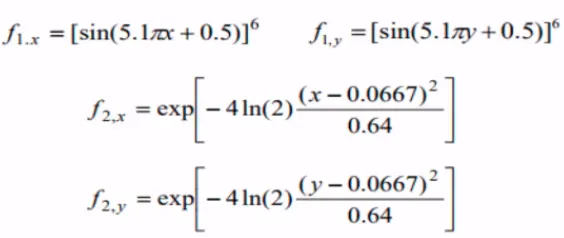
To optimise the stalagmite function and find the global maxima of the function given as

where
Main Code :
MAIN FUNCTION
-------------------------------------------------------------------------------
-------------------------------------------------------------------------------

clear all
close all
clc

%defining our search space
x=linspace(0,1,50);
y=linspace(0,1,50);
[xx yy]= meshgrid(x,y);
a=[xx yy];

cases=50;

tic
%case 1 - Studying statistical behaviour
for i=1:length(xx)
    for j=1:length(yy)
    input_vector(1)=xx(i,j);
    input_vector(2)=yy(i,j);
    f(i,j)=stalag_func(input_vector);
    end
end

for i=1:cases
    [inputs,fopt(i)]=ga(@stalag_func,2);
    xopt(i)=inputs(1);
    yopt(i)=inputs(2);
end

study1_time=toc

figure(1)
subplot(2,1,1)
hold on
surfc(xx,yy,-f)
shading interp
plot3(xopt,yopt,-fopt,'marker','o','markersize',5,'markerfacecolor','r')
title('Unbounded inputs')
subplot(2,1,2)
plot(fopt)
xlabel('Iterations')
ylabel('Function maximum')


%#Case 2- Studying statistical behaviour with upper and lower bounds
for i=1:length(xx)
    for j= 1:length(yy)

            %defining inputs for stalagmite function
            input_vector(1)=xx(i,j);
            input_vector(2)=yy(i,j);

            %obtaining stalagmite function values
            f(i,j)=stalag_func(input_vector);


    end
end

    for i=1:length(xx)

        [inputs,fopt(i)]=ga(@stalag_func,2,[],[],[],[],[0;0],[1;1]);

                xopt(i)=inputs(1);
                yopt(i)=inputs(2);


    end


study2_time=toc

figure(2)
subplot(2,1,1)
hold on
surfc(xx,yy,-f)
shading interp
plot3(xopt,yopt,-fopt,'marker','o','markersize',5,'markerfacecolor','r')
title('Bounded inputs')
subplot(2,1,2)
plot(fopt)
xlabel('Iterations')
ylabel('Function maximum')

%case 3- Increasing GA iterations

options=optimoptions('ga');
options=optimoptions(options,'PopulationSize',100);
for i=1:length(xx)
    for j= 1:length(yy)

            %defining inputs for stalagmite function
            input_vector(1)=xx(i,j);
            input_vector(2)=yy(i,j);

            %obtaining stalagmite function values
            f(i,j)=stalag_func(input_vector);


    end
end

    for i=1:length(xx)

        [inputs,fopt(i)]=ga(@stalag_func,2,[],[],[],[],[0;0],[0.1;0.1],[],[],options);

                xopt(i)=inputs(1);
                yopt(i)=inputs(2);


    end


study3_time=toc

figure(3)
subplot(2,1,1)
hold on
surfc(xx,yy,-f)
shading interp
plot3(xopt,yopt,-fopt,'marker','o','markersize',5,'markerfacecolor','r')
title('Bounded inputs')
subplot(2,1,2)
plot(fopt)
xlabel('Iterations')
ylabel('Function maximum')
Sub-Function:-
SUB-FUNCTION
--------------------------------------------------------------------------
--------------------------------------------------------------------------

function [s]= stalag_func(input_vector)
  %definition of functions in a stalagmite%
  m=input_vector(1);
  n=input_vector(2);
  f1x=(sin(5.1*pi*m+0.5))^6;
  f1y=(sin(5.1*pi*n+0.5))^6;
  f2x=exp((-4)*(log(2)*((m-0.0667)^2)/0.64));
  f2y=exp((-4)*(log(2)*((n-0.0667)^2)/0.64));
  s=(-1)*(f1x*f2x*f1y*f2y);
  end
Code explanation :
clear all
close all
clc
clears all the variables in the workspace which remain as residue, closes all active plots and clears the command window.
%defining our search space%
x=linspace(0,1,50);
y=linspace(0,1,50);
[xx yy]= meshgrid(x,y);
a=[xx yy];
Here, the search space has been defined.
%case 1 - Studying statistical behaviour
for i=1:length(xx)
for j=1:length(yy)
input_vector(1)=xx(i,j);
input_vector(2)=yy(i,j);
f(i,j)=stalag_func(input_vector);
end
end
for i=1:cases
[inputs,fopt(i)]=ga(@stalag_func,2);
xopt(i)=inputs(1);
yopt(i)=inputs(2);
end
study1_time=toc
figure(1)
subplot(2,1,1)
hold on
surfc(xx,yy,-f)
shading interp
plot3(xopt,yopt,-fopt,'marker','o','markersize',5,'markerfacecolor','r')
title('Unbounded inputs')
subplot(2,1,2)
plot(fopt)
xlabel('Iterations')
ylabel('Function maximum')
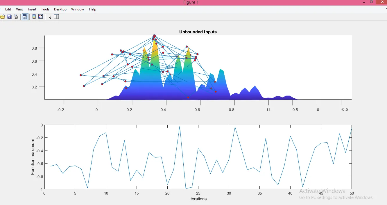
In case 1, statistical behaviour has been observed. Here, the fitness function values have been derived by giving input of search space, values of optimum x and y values have also been obtained by using loop iteratively. Using 'subplot' command, plots for studying the stalagmite curve and optimum solutions have been drawn on the same figure using suitable commands of 'plot' & 'plot3' and using suitable labels.
Note : '-f' and '-fopt' have been used so as to plot for maxima, since 'ga' works for finding a minima by default. Explanation for tweaking the stalagmite function has been given further, so as to find the maxima.
%#Case 2- Studying statistical behaviour with upper and lower bounds
for i=1:length(xx)
for j= 1:length(yy)
%defining inputs for stalagmite function
input_vector(1)=xx(i,j);
input_vector(2)=yy(i,j);
%obtaining stalagmite function values
f(i,j)=stalag_func(input_vector);
end
end
for i=1:length(xx)
[inputs,fopt(i)]=ga(@stalag_func,2,[],[],[],[],[0;0],[1;1]);
xopt(i)=inputs(1);
yopt(i)=inputs(2);
end
study2_time=toc
figure(2)
subplot(2,1,1)
hold on
surfc(xx,yy,-f)
shading interp
plot3(xopt,yopt,-fopt,'marker','o','markersize',5,'markerfacecolor','r')
title('Bounded inputs')
subplot(2,1,2)
plot(fopt)
xlabel('Iterations')
ylabel('Function maximum')
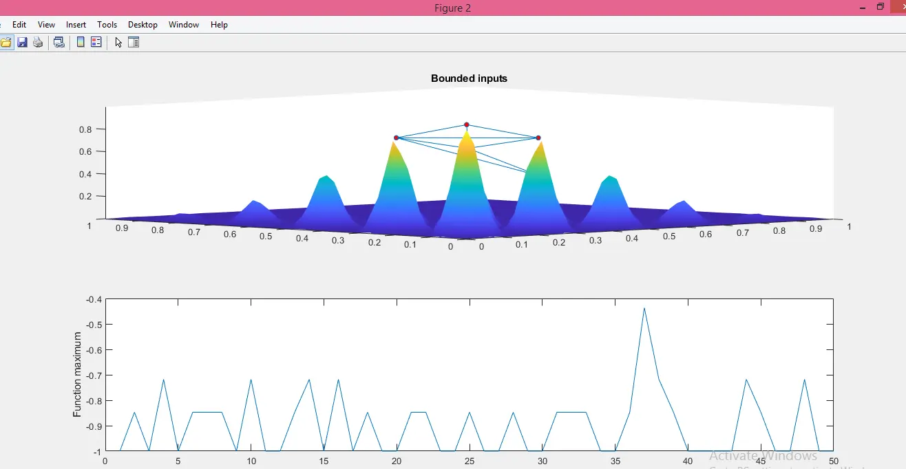
In case 2, the solution to find the maxima has been attempted with the syntax for 'ga' command with the mentioning of upper and lower bounds, which is [0;0] and [1;1] for x and y.
%case 3- Increasing GA iterations
options=optimoptions('ga');
options=optimoptions(options,'PopulationSize',100);
for i=1:length(xx)
for j= 1:length(yy)
%defining inputs for stalagmite function
input_vector(1)=xx(i,j);
input_vector(2)=yy(i,j);
%obtaining stalagmite function values
f(i,j)=stalag_func(input_vector);
end
end
for i=1:length(xx)
[inputs,fopt(i)]=ga(@stalag_func,2,[],[],[],[],[0;0],[0.1;0.1],[],[],options);
xopt(i)=inputs(1);
yopt(i)=inputs(2);
end
study3_time=toc
figure(3)
subplot(2,1,1)
hold on
surfc(xx,yy,-f)
shading interp
plot3(xopt,yopt,-fopt,'marker','o','markersize',5,'markerfacecolor','r')
title('Bounded inputs')
subplot(2,1,2)
plot(fopt)
xlabel('Iterations')
ylabel('Function maximum')
In case 3,
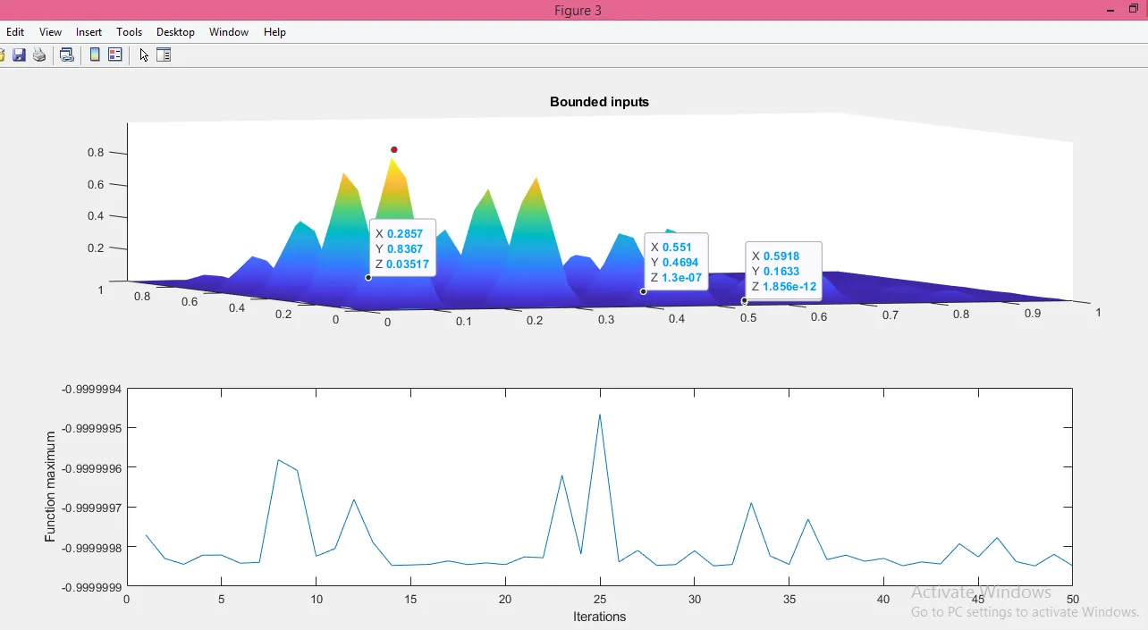
an attempt for finding the maxima has been made by increasing the population size to 100, following the syntax and changing the upper and lower bounds to [0;0] to [0.1;0.1] so as to fine tune the plots.
Sub-function explanation:-
function [s]= stalag_func(input_vector)
%definition of functions in a stalagmite%
m=input_vector(1);
n=input_vector(2);
f1x=(sin(5.1*pi*m+0.5))^6;
f1y=(sin(5.1*pi*n+0.5))^6;
f2x=exp((-4)*(log(2)*((m-0.0667)^2)/0.64));
f2y=exp((-4)*(log(2)*((n-0.0667)^2)/0.64));
s=(-1)*(f1x*f2x*f1y*f2y);
end
Here, the sub-function takes 'input_vector' as input search space. The individual functions have been defined and finally, the stalgmite function has been defined with addition of '(-1)' because 'ga' finds the minima by default and to convert into maxima, the curve must be inverted.
Output graphs:-
Case 1
Case 2
Case 3
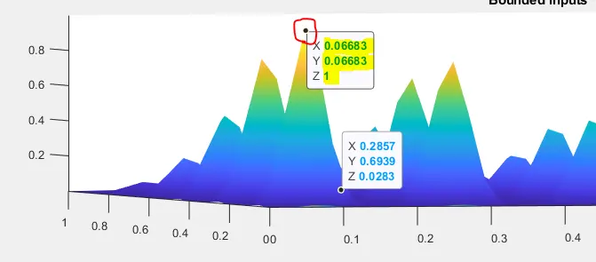
Point of Maxima :-
From the case 3 plot, it is aparent that the point of maxima occurs at (x,y) = (0.6683,0.6683)
and the objective function value (z) = (1)
Errors in code :
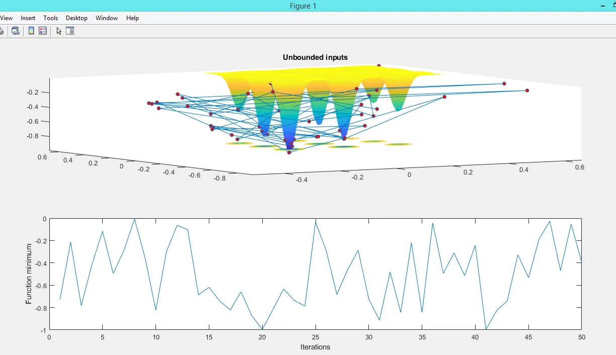
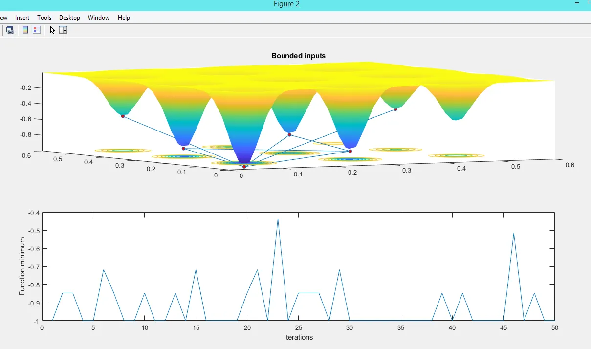
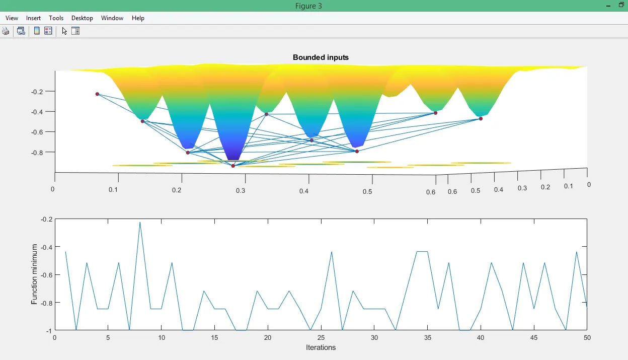
As apparent, the plots have not been reversed and axis labels are wrong. Also, the population size is as default.
Correction : In plot command, '-f' and '-fopt' were updated, axis label was changed to 'Function maximum' and population size was increased to 100.