Challenge

Week 2 Air standard Cycle

SSwarup Prateek Biswal2 Aug 2021

Air standard cycle (Otto cycle) challenge :

A series of operations occurring in a certain order is termed as a cycle. In an ideal cycle, all accidental heat losses are not taken into consideration and the working substance is assumed to behave like a perfect ideal gas. In an air standard cycle, the calorific value of fuel is altogether eliminated and the working substance is assumed to be air, hence the name Air standard cycle.

Certain assumptions made in the cycle :

The gas in consideration is a perfect gas, i.e, it is a perfect gas, obeys gas laws.
Physical constants of gas in the cylinder are the same as those of air at moderate temperatures i.e, Cp and Cv are constant throughout.
Compression and expansion processes are adiabatic, and take place without internal friction, i.e, the two processes are adiabatic.
No chemical reaction takes place in the cylinder. Heat is rejected by bringing a hot body or a cold body in contact with cylinder.
The same air is assumed to circulate in the engine.

Otto cycle or constant volume cycle, conceived by Nicolaus Otto, is a type of air standard cycle with heat exchange in the cycle taking place at constant volume.

Objective :

To write a code to solve an Otto cycle problem using Forward kinematics concept and plot PV diagram for the cycle and find the thermal efficiency of the engine.

Source code:

import math
import matplotlib.pyplot as plt


#geometric parameters
bore=0.1
stroke=0.1
con_rod=0.15
cr=12

def engine_kinematics(bore,stroke,con_rod,cr,start_crank,end_crank):
    #engine kinematics
    #Geometric parameters
    a=stroke/2
    R=con_rod/a
    
    #volume parameters
    v_s=math.pi*(1/4)*pow(bore,2)*stroke
    
    sc=math.radians(start_crank)
    ec=math.radians(end_crank)
    
    num_values=50
    v=[]
    
    dtheta=(ec-sc)/(num_values-1)
    
    for i in range(0,num_values):
        theta=sc+i*dtheta
        term1=0.5*(cr-1)
        term2=R+1-math.cos(theta)
        term3=pow(R,2)-pow(math.sin(theta),2)
        term3=pow(term3,0.5)
        v.append((1+term1*(term2-term3))*v_c)
        #print(v)
        
    return v
    
 #inputs
p1=101325
t1=500
gamma=1.4
t3=2300   
    
#volume computation
v_s = (math.pi/4)*pow(bore,2)*stroke
v_c  = v_s/(cr-1)
v1 = v_c + v_s

#state point2
v2=v_c    
    
#p2v2^gamma=p1v1^gamma
p2=p1*pow(v1,gamma)/pow(v2,gamma) 

#p1v1/t1=p2v2/t2=rhs|*| t2=p2v2/rhs
rhs=p1*v1/t1
t2=p2*v2/rhs

v_compression = engine_kinematics(bore,stroke,con_rod,cr,180,0)
#print(v_compression)

p_compression=[]

constant=p1*pow(v1,gamma)

for v in v_compression :
    p_compression.append(constant/pow(v,gamma))

#state point3
v3=v2

#p3v3/t3=rhs=p2v2/t2 |*| p3=rhs*t3/v3
rhs=p2*v2/t2
p3=rhs*t3/v3


v_exp = engine_kinematics(bore,stroke,con_rod,cr,0,180);

#print(v_exp)

p_exp=[]

constant=p3*pow(v3,gamma)

for v in v_exp :
    p_exp.append(constant/pow(v,gamma))

#state point4
v4=v1

#p4*v4^gamma=p3*v3^gamma
p4=p3*pow(v3,gamma)/pow(v4,gamma)

#p4v4/t4=rhs=p3v3/t3
t4=p4*v4/rhs

#thermal efficiency
eff= 1-((t4-t1)/(t3-t2))
print('Thermal efficieny is ',eff)

#plotting
plt.figure(1)
plt.plot([v1,v2,v3,v4,v1],[p1,p2,p3,p4,p1])
plt.xlabel('V ideal')
plt.ylabel('P ideal')

plt.figure(2)
plt.plot(v_compression,p_compression)
plt.plot([v2,v3],[p2,p3])
plt.plot(v_exp,p_exp)
plt.plot([v4,v1],[p4,p1])
plt.xlabel('V')
plt.ylabel('P')
plt.show()

Source code elaboration:

import math
import matplotlib.pyplot as plt

math library is imported as an alias.

bore=0.1

stroke=0.1

con_rod=0.15

cr=12

length of stroke, connecting rod, compression ratio and bore size are mentioned.

def engine_kinematics(bore,stroke,con_rod,cr,start_crank,end_crank):

Function named engine_kinematics has been defined passing arguments of bore size, stroke length, connecting rod length, compression ratio, crank start and end angles that shall be required to evaluate the volume matrix correspondingly for corresponding crank angle subtended. The mentioned function uses an iterative loop to evaluate the matrix of volumes.

The lines of code that follow in the function definition are :

a=stroke/2

R=con_rod/a

Defining a & R, as is

#volume parameters

v_s=math.pi*(1/4)*pow(bore,2)*stroke

Defining stroke volume mathematically

sc=math.radians(start_crank)

ec=math.radians(end_crank)

Defining start and end crank angles by converting them into angle in radians.

num_values=50

v=[]

dtheta=(ec-sc)/(num_values-1)

Defining dtheta variable and taking num_values number of iterations and setting v to a null vector.

for i in range(0,num_values):

theta=sc+i*dtheta

term1=0.5*(cr-1)

term2=R+1-math.cos(theta)

term3=pow(R,2)-pow(math.sin(theta),2)

term3=pow(term3,0.5)

(Breaking equations into different terms and defining as per equation )

v.append((1+term1*(term2-term3))*v_c)

(Using append function to store values of volume in each iteration)

return v

(Returning value of v matrix at the end of the loop)

#inputs

p1=101325

t1=500

gamma=1.4

t3=2300

(For state point 1, defining state variables of temperature, pressure)

#volume computation

v_s = (math.pi/4)*pow(bore,2)*stroke

v_c = v_s/(cr-1)

v1 = v_c + v_s

(Defining state stroke volume, compression volume, state point 1 volume mathematically)

#state point2

v2=v_c

#p2v2^gamma=p1v1^gamma

p2=p1*pow(v1,gamma)/pow(v2,gamma)

#p1v1/t1=p2v2/t2=rhs|*| t2=p2v2/rhs

rhs=p1*v1/t1

t2=p2*v2/rhs

(Defining state variables for state point1 & Deducing state point pressure and temperature at point 2 from gas equation for an adiabatic process)

v_compression = engine_kinematics(bore,stroke,con_rod,cr,180,0)

(Calling the user defined function engine_kinematics to evaluate the volume compression matrix by passing arguments for compression process in the cycle)

p_compression=[]

constant=p1*pow(v1,gamma)

for v in v_compression :

p_compression.append(constant/pow(v,gamma))

(Evaluating compression pressure matrix by setting the value to null and then calculating pressure at each point for corresponding volume governed by thermodynamic equation for an adiabatic process)

#state point3

v3=v2

#p3v3/t3=rhs=p2v2/t2 |*| p3=rhs*t3/v3

rhs=p2*v2/t2

p3=rhs*t3/v3

v_exp = engine_kinematics(bore,stroke,con_rod,cr,0,180);

(Calculating state point3 variables & calling the user defined function engine_kinematics to evaluate the expansion volume matrix by passing arguments for expansion process in the cycle)

p_exp=[]

constant=p3*pow(v3,gamma)

for v in v_exp :

p_exp.append(constant/pow(v,gamma))

v4=v1

#p4*v4^gamma=p3*v3^gamma

p4=p3*pow(v3,gamma)/pow(v4,gamma)

#p4v4/t4=rhs=p3v3/t3

t4=p4*v4/rhs

(Evaluating expansion pressure matrix by setting the value to null and then calculating pressure at each point for corresponding volume governed by thermodynamic equation for an adiabatic process. Calculating state point variables of temperature and pressure at point 4 from thermodynamic equations for an adiabatic process)

eff= 1-((t4-t1)/(t3-t2))

print('Thermal efficieny is ',eff)

(By definition, calculating the thermal efficiency)

#plotting

plt.figure(1)

plt.plot([v1,v2,v3,v4,v1],[p1,p2,p3,p4,p1])

plt.xlabel('V ideal')

plt.ylabel('P ideal')

plt.figure() lets us plot a new figure while plt.plot commands help plot the points as mentioned in the codes. Here, in the first figure, the plot is assumed to be ideal, i.e, the expansion and compression have been assumed to have taken place ideally. The plot has been labelled ideal pressure vs. ideal volume.

plt.figure(2)

plt.plot(v_compression,p_compression)

plt.plot([v2,v3],[p2,p3])

plt.plot(v_exp,p_exp)

plt.plot([v4,v1],[p4,p1])

plt.xlabel('V')

plt.ylabel('P')

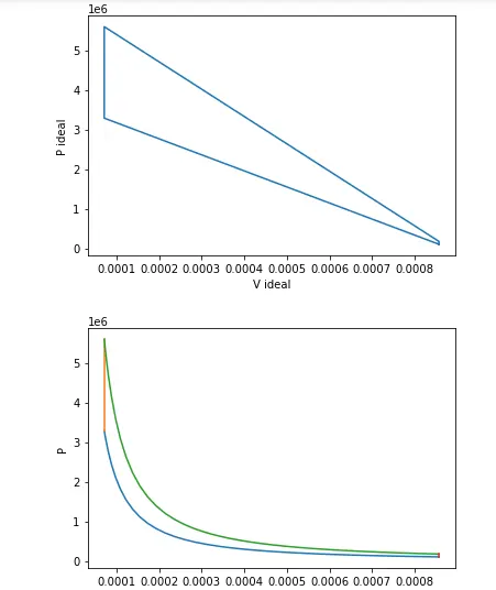
plt.figure() lets us plot a new figure while plt.plot commands help plot the points as mentioned in the codes. Here, in the second figure, the plot is assumed to be real, i.e, the expansion and compression have been assumed to have taken place ideally. The plot has been labelled pressure vs. volume. In order to plot the points, we have plotted the points in each step discretely. The adiabatic process has been plotted using the state point matrix.

plt.show()

plt.show(): shows all the files plotted in the file.

Output:

The output of the program is as follows:

For the given dataset, the thermal efficiency is found to be 0.6298 or 62.98%.

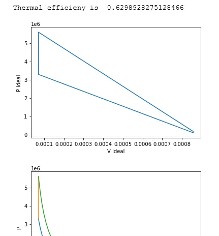
The ideal cycle and actual cycle PV diagrams are shown correspondingly.

Errors faced:

Errors faced during compilation of code are as follows:

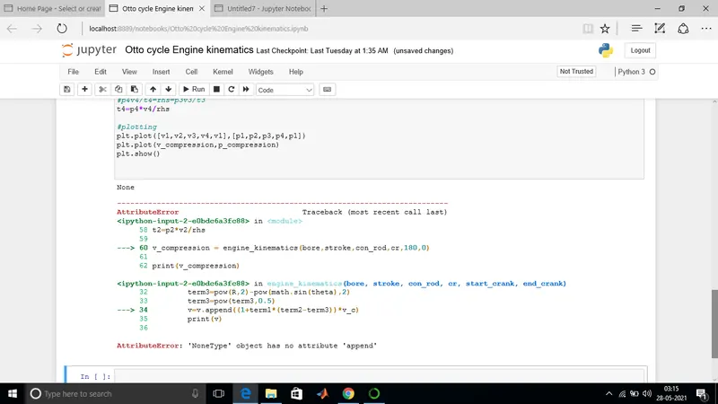
In one case, "Attribute error" was displayed for append being no attribute for 'NoneType' object.

Line code v=v.append((1+term1*(term2-term3))*v_c) caused the error

Corrective action for debugging the code:

The code was modified to v.append((1+term1*(term2-term3))*v_c) no error was thrown with value of v being stored correctly.

Sources: The following sources have been used for case study and arriving at a conclusion:

Week 2 Air standard Cycle

Ship work like this
in your own course.

Talk to a career counsellor

Ship work like thisin your own course.

Talk to a career counsellor

Ship work like this
in your own course.